
CASA News
Issue 4
11 October 2016

CASA News
Issue 4 • 11 October 2016

Letter from the Lead
Let me begin by welcoming our colleagues at the newly formed Academia Sinica Institute of Astronomy and Astrophysics (ASIAA) Common Astronomy Software Applications (CASA) Development Center (see article in this CASA News by Chin-Fei Lee). We welcome them to the collaboration and look forward to working with them in the coming years.
The Very Large Array (VLA) and Atacama Large Millimeter/submillimeter Array (ALMA) pipelines continue to mature and grow in capability. The ALMA interferometric imaging pipeline has been reworked in support of ALMA Cycle 4, and is expected to be used in producing images for many ALMA Cycle 4 projects. The VLA Sky Survey (VLASS) is gathering momentum as the targeted start during the next B-configuration is just under one year in the future. Development toward the calibration and imaging pipelines for VLASS is underway.
The CASA team has been continuing to address reliability, robustness, and usability issues. A major rework of the CASA documentation is underway, and is planned to be released with the CASA-5.0 release in March 2017.
The NRAO Users Committee recommended that the visibility of the CASA News be improved by distributing this issue to all NRAO eNews subscribers. If you wish to unsubscribe from CASA News, please visit the CASA News Information Page and fill out the unsubscribe section at the bottom of the page.
Helpdesk & User Support
Please help us help you! Since April 2016, we have received 219 tickets through our Helpdesk system, supporting CASA processing of VLA, ALMA, and other telescope data. When you need help, please send us as much information as you can about your computer, what you were doing to your data before the issue, information about the data you are working with, and any error messages generated from the issue. We can help you faster when we have as much information as possible.
Tell us about your computer.
Are you running CASA on your local machine or a remote server? If you are running remotely, are you using VNC or some other mechanism to access the remote machine? What operating systems are on the remote machine and the local machine? If you are using an Observatory-provided visitor account, tell us your account username. If you are on your local machine, check to see if your operating system is officially supported by the CASA project (see the Obtaining CASA web page for a list). Though unsupported operating systems may not cause problems, differences in system libraries can result in unexpected errors. Use a supported operating system if at all possible.
What you were doing to your data before the issue?
Measurement sets, in particular, can become corrupted under some circumstances, and when this happens no amount of expert advice will solve your problem. So tell us what you have done to your data since downloading it from the archive.
Describe your data.
Tell us what telescope acquired your data. If it is simulated data, tell us how you created the data. What kind of setup is your data (bandwidth switching, polarization, etc.)?
Provide all error messages.
Attach the CASA log file to your Helpdesk ticket. Doing so will help us better understand your particular data processing situation and enables us to reply more promptly. Copy over anything that was printed to the terminal and what parameter values you used when running a task. Include the CASA version (e.g., Release 4.6.0) you are using when you submit your ticket. If you are not using the latest CASA version, try upgrading first. The CASA developers are continually addressing bugs and adding new features, and it is possible your issue has been addressed in a recent CASA release.
Please also feel free to send us feedback on either CASA or the Helpdesk. We are currently working on implementing the ability for users to reply to Helpdesk tickets via email, as requested by the users. You can provide feedback in your existing CASA ticket or open a new ticket in the “General Queries” Helpdesk department.
Please keep those Helpdesk questions coming!
CASA Calendar
| Date | Event |
|---|---|
| 30 Sep 2016 | Start of ALMA Cycle 4 Observing |
| 9-14 Oct 2016 | SKA Calibration and Imaging Workshop, Socorro, New Mexico, USA |
| 17-20 Oct 2016 | Coexisting with Radio Frequency Interference, Socorro, New Mexico, USA |
| 1 Feb 2017 | NRAO Semester 2017B Observing Proposal Deadline |
ASIAA CASA Development Center

On 1 August 2016, the Academia Sinica, Institute of Astronomy and Astrophysics (ASIAA) established the ASIAA CASA Development Center (ACDC), in collaboration with NRAO. The primary goals of this collaboration are to increase our international collaboration and visibility, advance our high-performance computing techniques and software engineering, and raise our science productivity from ALMA and other radio interferometer observations.
Development at the ACDC will be fully integrated and coordinated with the CASA team. For the initial year, the ASIAA team will augment the NRAO effort on the next generation CASA image viewer: Cube Analysis and Rendering Tool for Astronomy (CARTA). In the second year, the ASIAA center will add a component of high performance computing (HPC) to the development targets. This work will be coordinated with the overall CASA HPC strategy and may include aspects of resource management (memory management and persistent storage bandwidth utilization) in addition to parallelization, and compute optimization.
msuvbin: a task for uv data averaging
There is an experimental task in CASA called msuvbin. The main purpose of this task is to average or bin uv data. Users who have several observations on the same target with overlapping spectral parameters may find this task useful. The output data set is fixed in size. The user's needs determine ahead of time parameters such as the extent of the field-of-view, the highest spatial resolution, the frequency coverage, and the best spectral resolution that will ever be needed from the data sets that are to be binned and combined. These parameters will then determine the size of the output data set.
When doing spectral channel averaging, the uv-value of each channel being binned into a spectral bin is accounted for and, therefore, bandwidth decorrelation will not occur. If the field-of-view of interest is large enough that w-term corrections (w-projection) are needed, then msuvbin can be made to perform these corrections while binning the data. The only limitation while using w-projection is that, at present, the task clean cannot be run on the w-term binned uvdata with multiple Cotton-Schwab cycles while making the image or the image cube. One should just invert the visibilities and then use a deconvolver on the dirty image.
Additional details are available in EVLA memo 198.
Commissioning Effort for Wide-field, Wide-band Imaging
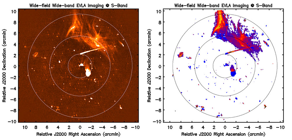
Wide-field wide-band continuum imaging of the A2256 field at S-Band with the VLA. [Left] Stokes-I image. [Right] Intensity weighted spectral-index map. The contours show the antenna primary beam at the 90, 50 and 10 % levels.
[click to enlarge]
Imaging the full wide-band sensitivity pattern is required for accurate continuum imaging with widespread emission, e.g., at the VLA "low bands" where the sky brightness distribution is both strong and widespread or for mosaic imaging, in general, where the instrumental effects affect the entire mosaic field.
Wide-field, wide-band imaging requires corrections for instrumental direction-dependent effects like the time, frequency, and polarization dependence of the antenna far-field power pattern, as well as accounting for intrinsic frequency dependence of the sky brightness distribution. In CASA, this is done using a combination of the Multi-term Multi-Frequency Synthesis (MT-MFS, Rau & Cornwell) and Wide-band AW-Projection (WB-AWP) algorithms. The MT-MFS algorithm, available in CASA releases, models the sky brightness as a function of frequency in the image modeling (a.k.a. "deconvolution") process. The WB-AWP algorithm (Bhatnagar et al.) corrects for the variations of the antenna far-field power pattern in time, frequency, and polarization as well for the effects of non-coplanar baselines in the process of imaging the visibility data. The combined MT-MFS and WB-AWP algorithms enables wide-field wide-band imaging throughout the antenna wide-band field-of-view and the mosaic pattern for joint-mosaic imaging.
The WB-AWP relies on an accurate wide-band model for the antenna aperture illumination pattern. Since the compute-load and the memory footprint of the combined algorithm is intrinsically significantly higher, from the point-of-view of run-time, it becomes important to also enable wide-field, wide-band imaging using parallel processing. This significantly increases the algorithmic and software complexity.
The Algorithm Research & Development personnel in CASA have been working with a few advanced users for commissioning the wide-field wide-band imaging capability. The existing implementation has been applied to real data from the VLA and the Stokes-I and Spectral Index maps carefully tested for correctness. This effort is also simultaneously commissioning the general parallel-processing framework for continuum imaging in CASA. As part of this effort, we recently re-imaged the Abell 2256 (A2256) field at S-band using CASA, where the emission of interest spans the full field-of-view.
The image on the left in Figure-1 shows the resulting Stokes-I image with the overlaid contours showing the antenna gain pattern at 90, 50, and 10% levels. The image on the right shows the intensity-weighted Spectral Index map of the same field with recovered sky spectral index ranging from -0.7 (blue) to -2.5 (red/yellow). Emission that shows up in blue color (spectral index ~ -0.7) in this image is spread across the field, indicating that the effects of the antenna gain pattern, particularly as a function of frequency has been largely corrected. Without correcting for the frequency dependence of the antenna gain, a secular increase in the spectral index with distance from the center would result.
This is an on-going effort and as a result, a number of issues have been found, and some have been fixed. Outstanding issues include non-repeatable crashes (probably only when run in parallel) and residual effects of frequency dependence of the antenna gain pattern which increases the error on the recovered spectral index with distance from the center of the beam. This could come from a variety of sources including the model for the antenna gain pattern used and / or subtle numerical issues in the implementation. Ongoing efforts are underway to understand these and other issues related to deploying the code on HPC platforms exposed via the current commissioning initiative.
References:
MT-MFS (Rau & Cornwell, A&A, Vol. 532, Aug. 2011)
WB AW-Projection (Bhatnagar, et al., (2013,Vol.770, No. 2, 91))
eXtended CASA Line Analysis Software Suite (XCLASS)
The eXtended CASA Line Analysis Software Suite (XCLASS) is a toolbox for CASA containing new functions for modeling interferometric and single dish data. It produces physical parameter fits for all molecules in a dataset. This also allows line identification, but provides much more information.
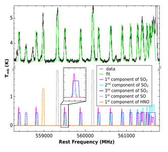
Figure 1: Here, the myXCLASS function was used to model HIFI data of Sgr B2(M) (black) using SO2 (with three different components), SO (with one component), and HNO (with one component). The intensities of each component are shown in the bottom half.
[click to enlarge]
The philosophy behind XCLASS is to work on the species level rather than on individual lines. All lines of a species in a given data range are fitted simultaneously with a physical model, which reduces the risk of mis-assignments due to blends, and allows for robust identifications of species. This is because the method allows checking that all lines that should be there are there, with the expected strength. For this purpose, XCLASS models a spectrum by solving the radiative transfer equation for an isothermal object in one dimension (detection equation) assuming LTE. That means that the source function is given by the Planck function of an excitation temperature, which is constant for all transitions, but not necessarily equal to the kinetic temperature. XCLASS is designed to describe line-rich sources which often have high densities, so that LTE is a reasonable approximation. Also, a non-LTE description requires collision rates which are available only for a few molecules. Molecular data required by this function are taken from an embedded SQLite3 database containing entries from the Cologne Database for Molecular Spectroscopy (CDMS) and the Jet Propulsion Laboratory (JPL) using the Virtual Atomic and Molecular Data Center (VAMDC) portal. This database has more entries for the partition function, 100 between 1 and 1000 K, than the standard CDMS/JPL catalog entries, which avoids hazardous extrapolation for low excitation temperatures, e.g., for absorption lines. XCLASS is able to model a spectrum with an arbitrary number of molecules where the contribution of each molecule is described by an arbitrary number of components (see Figure 1). Here, each component is described by the source size, the temperature, the column density, the velocity width and offset, which has to be defined by the user in the input file.
Due to the large number of input parameters required by XCLASS, it is essential to use a powerful optimization package to achieve a good description of observational data. Therefore, XCLASS contains the MAGIX package which is a model optimizer providing an interface between existing codes and an iterating engine. The package attempts to minimize deviations of the model results from observational data with a variety of algorithms, including swarm algorithms to find global minima, thereby constraining the values of the model parameters and providing corresponding error estimates. Besides the myXCLASS function to produce synthetic spectra, XCLASS includes two additional functions – myXCLASSFit and myXCLASSMapFit – which provide a simplified interface for MAGIX using XCLASS.
The myXCLASSFit function offers the possibility to fit multiple frequency ranges in multiple files from multiple telescopes simultaneously using MAGIX in conjunction with myXCLASS. The function returns the optimized molfit file and the corresponding modeled spectra.
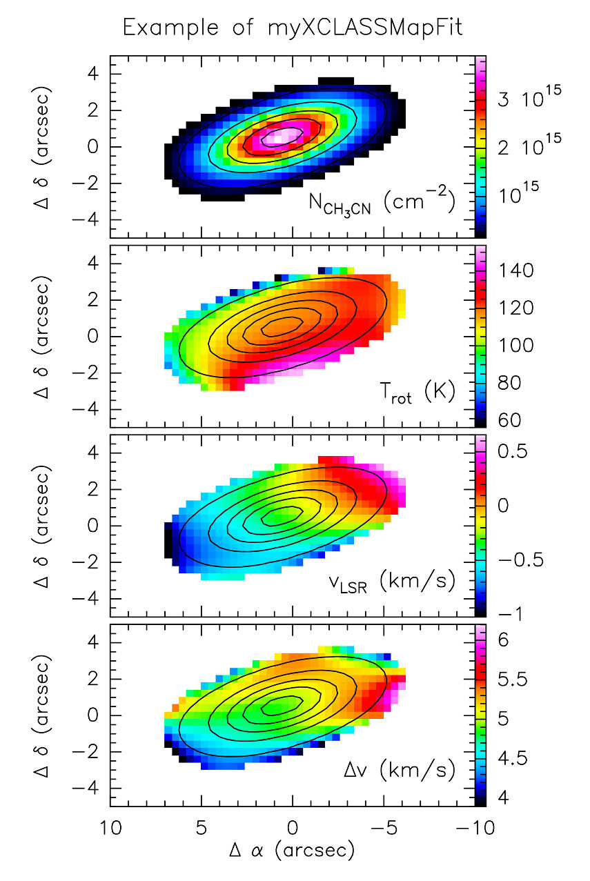
Figure 2: Example of parameter maps created by the myXCLASSMapFit function. Here, the K-ladder structure of the CH3CN (12-11) transition (plus isotopologues) in G75.78+0.34 was fitted at around 220 GHz (observed with the SMA). The temperature gradient is expected as also seen in different NH3 lines (Sanchez-Monge et al.)
[click to enlarge]
In addition to the myXCLASSFit function, which is useful to fit single spectra, the XCLASS interface contains the myXCLASSMapFit function which fits one or more complete (FITS) data cubes. For this, the myXCLASSMapFit function reads in the data cube(s), extracts the spectra for each pixel and fits these spectra separately. It offers the possibility to limit the fit to certain frequency ranges of a spectrum and to a user-defined region of the cube(s). To reduce the computation effort, the user can exclude pixels by defining a threshold for the minimum intensity of a pixel to be fitted.
At the end of the fit procedure, the myXCLASSMapFit function creates FITS images for each free parameter of the best fit, where each pixel corresponds to the value of the optimized parameter taken from the best fit for this pixel, see Figure 2. Furthermore, the myXCLASSMapFit function creates FITS cubes for each fitted data cube, where each pixel contains the modeled spectrum. Finally, the myXCLASSMapFit function creates one FITS image which describes the quality of the fit for each pixel. Here, each pixel corresponds to the χ2 value of the fit for this pixel.
Applications of this are temperature maps, but also first and second moment maps, which are based on the simultaneous fitting of many lines, and are fairly robust against line confusion and blending of single lines, which is a severe issue in many ALMA data sets of line-rich sources.
We acknowledge support from VBF/BMBF Projects 05A11PK3 and 05A14PK1 for the German ARC Node, and from the ESO ALMA development project 56787/14/60579/HNE.
The software and a manual are available on-line.
CASA on Amazon Web Services
The NRAO is pleased to announce new on-line documentation covering the use of Amazon Web Services (AWS) computing resources for processing data with the Common Astronomy Software Applications (CASA) package. AWS is a collection of physical assets and software tools for using ad hoc computing resources (cloud computing) within Amazon. The combination of a wide range of processing hardware, network speeds, storage media, and tools allows users to create virtual computing platforms tailored to specific problem sizes.
AWS has the potential to provide substantial time savings via distributed processing across more resources than are typically available. NRAO has successfully run a simulation across 1000 AWS servers, e.g., reducing a 4000-hour duration serial execution to a 4+ hour parallel run. Because AWS charges on a per use basis, it may provide a cost savings for anyone investigating acquiring new hardware that would only experience periodic usage.
The new documentation covers the basics of AWS usage, resource selection, and cost considerations in the context of CASA-based processing and includes pointers into the vast AWS documentation repository. Over time, the documentation will be expanded to include more complex use cases and example scripts for automation.
As this is a new processing model, and given the unique nature of AWS resources, please direct any questions or comments to nrao-aws@nrao.edu rather than to CASA or Helpdesk personnel.
Those acquiring their own computing should review the hardware recommendations page which has been updated to reflect newly available hardware including the new Intel line of multi-TB, high-speed, Non-Volatile Memory Express (NVMe)-based solid-state drives.
CASA-based Pipelines
Figure 1: Image of ALMA band 7 science verification data of HL Tau. [Left] Cycle 3 pipeline result with simple imaging parameters leading to under cleaning. [Right] Cycle 4 pipeline result with new threshold and iteration heuristics enabled. The cleaning is much better due to more realistic sensitivity limits.
[click to enlarge]
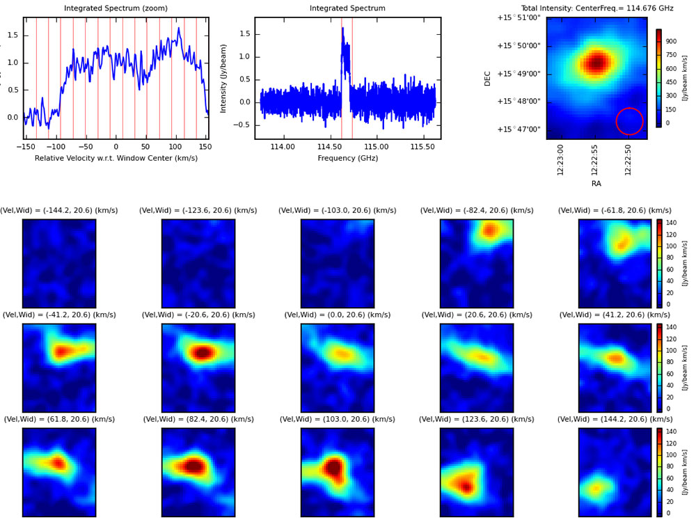
Figure 2: Channel maps of ALMA band 3 single dish science verification data of M100 processed by single dish PIPELINE. [Top Right] Integrated intensity (moment 0) image. [Top Center] The spectrum integrated over the map area. The red vertical lines indicate the lower and upper limits of frequencies of a spectral line detected by PIPELINE. [Top left] Zoom up of the frequency range of spectral line. Red vertical lines indicate boundaries of frequency ranges of channel maps in lower panels.
[click to enlarge]
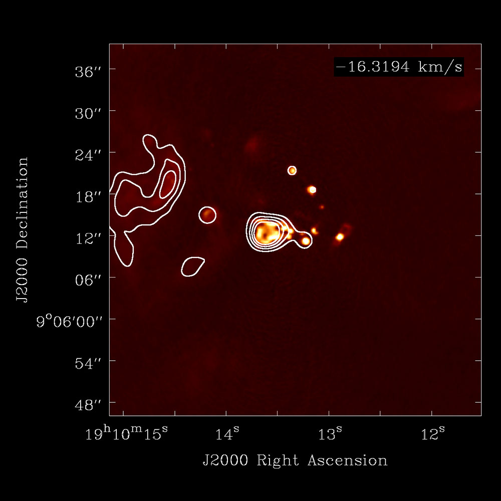
Figure 3: This Jansky VLA data of galactic source W49 was calibrated with the pipeline and then imaged by Chris DePree, Terry Melo, and Kira Fritsche (Agnes Scott College) while testing the new spectral line heuristics. The heat map continuum image at 9.817 GHz (H87α) is from all four Jansky VLA configurations. Line emission is clearly detected in the H88α data (overlay contours) with C-configuration.
[click to enlarge]
The past six months have been busy ones for the pipeline team. Pipeline activities have concentrated on: development and testing of the ALMA interferometry and single dish pipeline releases for Cycle 4, upgrades to the Jansky VLA calibration pipeline, and assessment of the development effort required to support the VLA Sky Survey (VLASS) pipelines.
ALMA interferometry pipeline development for Cycle 4 focused on improvements to the the Cycle 3 informative imaging pipeline. New imaging pipeline features include: an updated imaging workflow and standard recipe, improved science target continuum frequency range identification heuristics, new tasks for science target continuum fitting and subtraction, improved continuum and cube sensitivity estimation heuristics, improved dynamic range based cleaning iteration and threshold determination heuristics, and improved quality assessment metrics for all pipeline generated images. The Cycle 4 release also supports new gain calibration based flagging heuristics and new low signal to noise gain calibration heuristics. The combined effect of the Cycle 3 to Cycle 4 flagging, calibration, and most significantly, the imaging heuristics improvements are illustrated in Figure 1 below.
ALMA 4 single dish pipeline development for Cycle 4 focused on replacing the Australian Telescope National Facility (ATNF) Spectral Analysis Package (SAP) table format with the native CASA measurement set format, adding support for multi-source execution blocks, improving intent based data selection, and developing new tasks for applying the calibrations to the data. These changes have significantly improved the single dish pipeline processing efficiency. They have also helped unify the pipeline framework code and enabled more code sharing with the ALMA interferometry pipeline. Representative image(s) produced by a recent single dish run are shown in Figure 2 below.
Jansky VLA calibration pipeline development has focused on developing low signal-to-noise bandpass calibrator heuristics and adding support for spectral line projects to the Hanning smoothing, science target flagging, and weights computation tasks via a spectral line regions file. A representative image constructed from a recent, pipeline calibrated spectral line project is shown in Figure 3.
Development of the pipeline framework, which is shared by all three operational pipelines also continued over the past six months. Most recent major improvements were driven by the needs of VLASS and the availability of early VLASS data. VLASS data is acquired in On-The-Fly (OTF) mode. OTF data acquisition results in data sets with an unusual structure compared to standard ALMA and VLA data sets. Each VLASS data set, e.g., contains thousands of fields. This data structure revealed serious shortcomings in the pipeline and CASA metadata handling code and in the pipeline calibration library code. These issues have already been addressed and resulted in major efficiency improvements to the pipeline framework.
Testing of the pipeline / CASA HPC framework is ongoing. All three operational pipelines do run in HPC mode, but pipeline / HPC operations are not yet routine. The pipeline has also been run successfully in the cloud via Amazon Web Services.
There have been three pipeline test releases in the past six months. The latest is C4R2.1 which will be delivered as part of CASA 4.7. Once the C4R2.1 release is deployed and operational, new pipeline development will resume. Over the next 6 months, ALMA development will focus on adding support for observing sessions and sharing calibration observations across execution blocks, and on the imaging and quality assessment code cleanup. VLA development will focus on adding polarization calibration heuristics to the calibration pipeline and on developing imaging heuristics for the VLASS pipeline.
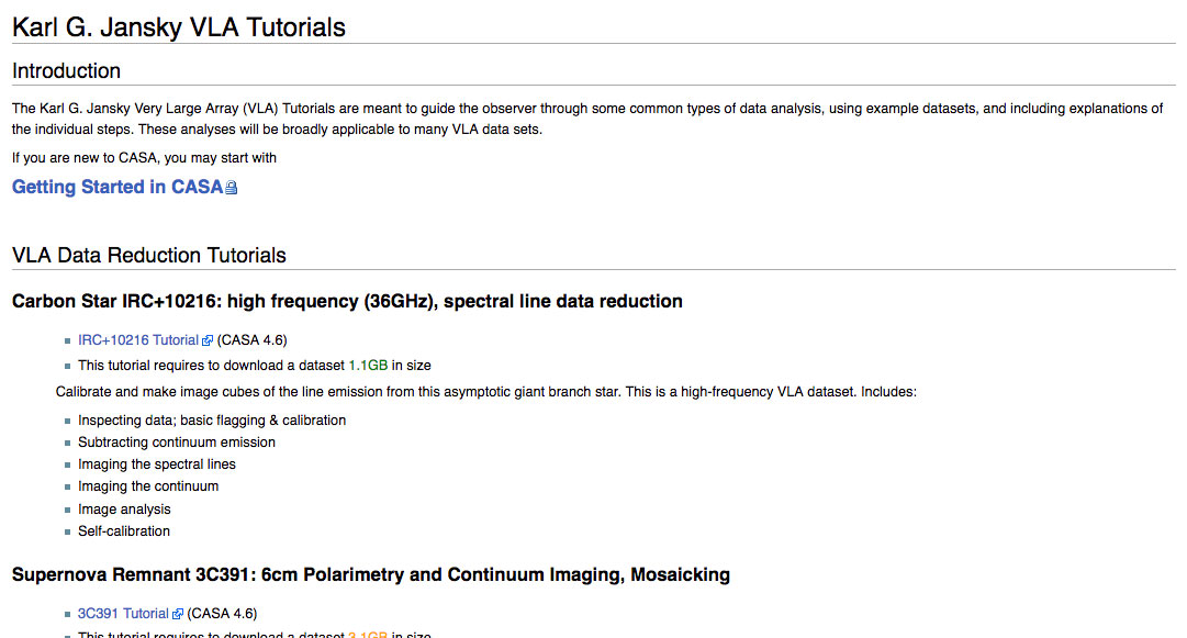
New VLA CASA Guides
[click to enlarge]
CASA guides are tutorials that provide recipes for typical data reduction paths for various telescopes. In the last few months, we have restructured the CASA guides for Very Large Array (VLA) data reduction. This includes new topical guides as well as a new VLA pipeline guide.
Full data reduction steps are provided via three CASA guides, summarized below, that are kept up-to-date with the latest CASA versions.
- IRC+10216: A high frequency spectral line tutorial that explains the individual calibration steps, continuum subtraction, cube imaging, spectral line analysis methods, and provides a brief self-calibration demonstration.
- 3C391: A 7-pointing mosaic continuum tutorial using C-band data for polarization calibration and full Stokes (I, Q, U, V) imaging. It also includes spectral index analysis and self-calibration.
- P-band tutorial: This guide illustrates typical sub-GHz calibration steps including ionospheric calibration and polarization calibration for the linear feeds.
In addition, we now offer the following self-contained, topical CASA guides for the VLA.
- Flagging: This guide includes radio-frequency-interference (RFI) identification, manual editing, and automatic RFI excision algorithms.
- Imaging: An introduction to clean and its options such as multi-scale, wide-field, and multi-term algorithms, outlier fields, primary beam correction, and a brief description of spectral cube imaging.
- Spectral Index Correction for Bandpass Calibration: This short guide describes how to correct the bandpass shape if the spectral index of the bandpass calibrator is not known.
- VLA CASA Pipeline: This guide describes how to execute the VLA CASA calibration pipeline and discusses its products. It outlines the weblog and presents how plots and calibration tables should be interpreted. This guide concludes with examples on modifying and re-running the pipeline, as well as editing the scan intents when needed.
- (Coming soon) Data combination: a VLA CASA recipe to combine data from different observations and array configurations.
All CASA guides are available from the Karl G. Jansky Very Large Array CASA guides page and will be updated as new CASA and VLA pipeline releases become available.
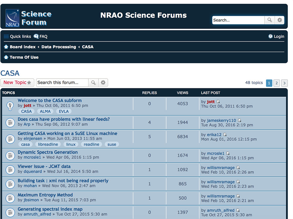
CASA Forum
[click to enlarge]
In addition to the CASA Helpdesk, we also have a CASA Forum. The CASA Forum is part of the NRAO Science Forums and provides a place where CASA issues can be discussed. Although CASA staff may occasionally contribute, the forum is meant to facilitate exchanges between CASA users and friends. Do you want to ask your colleagues about data reduction techniques that are not part of standard CASA? Try the Forum. Do you have a script that you want to share? Try the Forum. Do you have python questions? Try the Forum. Do you have data from telescopes that are not officially supported? Try the Forum. Are you trying to use CASA on an unsupported operating system? Try the Forum.
The CASA Forum can be viewed by anyone, but to avoid spamming we ask every contributor to log in with their my.nrao.edu credentials. If you have specific questions that you want a CASA staff member to address, please submit them to the CASA Helpdesk. For everything else, users on the CASA Forum may provide some help.
We look forward to lively discussions!