
CASA News
Issue Iss#
Day# Month# Year#

CASA News
Issue Iss# • Day# Month# Year#

Letter from the Lead
It has been a year since our last newsletter update to the Common Astronomy Software Applications (CASA) community. In that time, much has changed in the world that impacts the way we all live and work. The diverse and global nature of the CASA team has affected everyone differently. Many contributing organizations–including NRAO, ESO and NAOJ–have been working partially or wholly remote for the past seven months. The ALMA telescope and JAO offices in Chile have been closed as well. The CASA team has had to adapt to this new environment and look for ways to modernize and improve our technology base. As the current situation looks likely to continue in many parts of the world for the foreseeable future, we continue to develop CASA releases as best we can while embracing changes to better support the reality we all now find ourselves in.
Despite the inefficiencies and setbacks that have come from the global shutdowns, we are pleased with the accomplishments of the last year, including the CASA 6.1 release, joint single dish / interferometer image reconstruction, new processing techniques for the VLA Sky Survey, and prototyping efforts on a new next-generation CASA infrastructure.
CASA 5.7 / 6.1
The CASA Team is pleased to announce that CASA 5.7/6.1 has been released. CASA 6.1 is the first modular pip-wheel version of CASA 6 (Python 3) that is supported for our general user community. CASA 5.7 and 6.1 feature the same new development, while CASA 5.7 is based on Python 2 and CASA 6.1 is based on Python 3. CASA 6.1 is available either as a downloadable tar-file (like CASA 5.7 and earlier versions), or through pip-wheel installation, which gives users the flexibility to integrate CASA into their own Python environment. More information is available in CASA Docs.
As described elsewhere in this Newsletter, a major new addition to CASA 5.7/6.1 is the introduction of a new task for joint deconvolution of single-dish and interferometry data, sdintimaging. This has been a major priority for our user base, and we are pleased to announce that this algorithm provides great improvement in combining single-dish and interferometry data across a range of use-cases that we have tested and documented in CASA Docs. Further testing and implementation of this joint deconvolution algorithm is ongoing.
Other highlights include:
- For single-dish processing, a new task sdtimeaverage is available for averaging single-dish spectral data over specified time.
- A new single-dish spectral imaging mode, 'cubesource', is available in the task tsdimaging to perform spectral imaging of moving sources.
- Parameter corrdepflags has been added to the gaincal, bandpass, and fringefit tasks to permit more control of flagging subsets of correlations.
- The ability to correct for heterogeneous antenna pointing offsets has been added to tclean.
- Additional improvements have been made to the statwt task.
- The fringefit task now includes support for dispersive delays.
- The CASA simulator has transitioned to tclean, paving the way to deprecate clean. In addition, simobserve now reads and populates antenna names rather than assigning numbers, improving its user-friendliness.
- VLA P-band models have been made available in CASA for several standard calibrators, and ephemeris tables for Solar System objects have been extended in time.
In addition, version 1.4 of the CARTA visualization software has been released, as described elsewhere in this Newsletter. Also, a large number of user-facing bugs in CASA have been fixed, and our test modules have been progressively extended to increase reliability of CASA. The full list of new functionality in CASA 5.7/6.1 can be found in the Release Notes on CASA Docs.
CASA 5.7 / 6.1 can be downloaded here.
We welcome any feedback from users on this new version of CASA.
Joint Image Reconstruction using Interferometer and Single Dish data
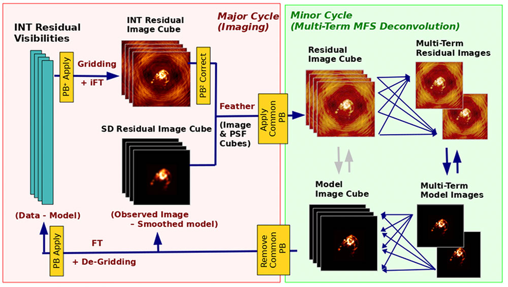
Fig. 1: Schematic overview of the algorithm for joint deconvolution of single dish and interferometry data.
[click to enlarge]
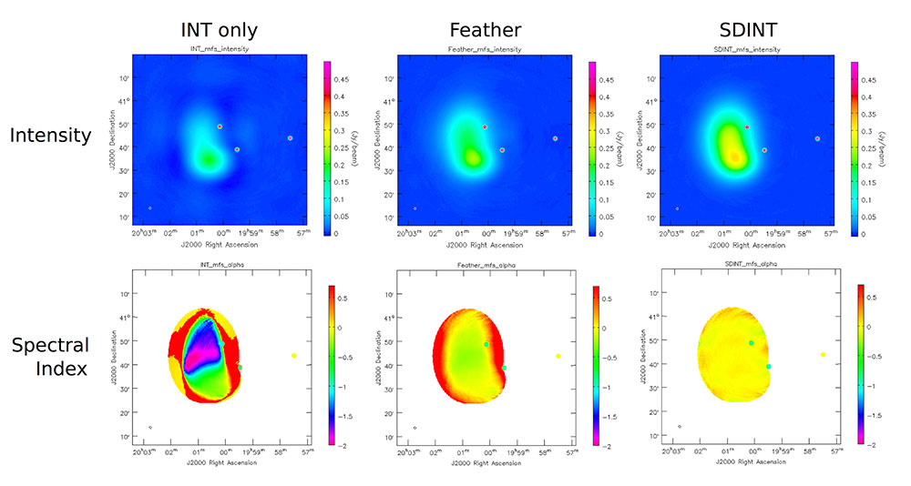
Fig. 2: Example of joint deconvolution applied to simulated wideband data sets.
[click to enlarge]
Overview
CASA 6.1/5.7 introduces a new task, sdintimaging, to perform joint reconstruction of wideband single dish and interferometer data. The sdintimaging task implements the algorithm published in Rau, Naik & Braun, 2019 with the CASA implementation documented via the SDINT task interface and a summary page containing examples and verified usage modes.
The sdintimaging task supports joint deconvolution for spectral cubes as well as multi-term wideband imaging, operates on single pointings as well as joint mosaics, includes corrections for frequency dependent primary beams, and optionally allows the deconvolution of only single-dish images in both cube and multi-term mfs modes. An option has also been provided to tune the relative weighting of the single dish and interferometer data alongside the standard weighting schemes used for interferometric imaging. Our initial results demonstrate the ability to prevent instabilities and errors that typically arise when wideband or joint mosaicking algorithms are presented with spatial and spectral structure that is inadequately sampled by the interferometer alone. For CASA 6.1, this task has been released as 'experimental' and is currently intended for the exploration of the algorithm's capabilities and to gather feedback for the further refinement of the interface.
Algorithm
Interferometer data are gridded into an image cube (and corresponding PSF). The single dish image and PSF cubes are combined with the interferometer cubes in a feathering step, using CASA’s feather task. The joint image and PSF cubes then form inputs to any deconvolution algorithm (in either cube or mfs/mtmfs modes). Model images from the deconvolution algorithm are translated back to model image cubes prior to subtraction from both the single dish image cube as well as the interferometer data to form a new pair of residual image cubes to be feathered in the next iteration. In the case of wideband mosaic imaging (cube or mfs), wideband primary beam corrections are always performed per channel of the image cube, followed by a multiplication by a common primary beam, prior to deconvolution.
Example
Imaging results from a wideband simulation are shown in Figure 2. The true sky brightness consists of flat-spectrum extended structure approximately matched in scale to the central unsampled region of the interferometer data, and three point sources (two of which have steep spectra and one which is flat). The panels below show intensity and spectral index maps made with interferometer-only data (left), feathered images (middle) and a joint reconstruction (right) and show progressively more accurate reconstructions of both the intensity distribution and large-scale spectral index.
Next-Generation CASA
[click to enlarge]
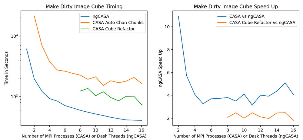
Standard Gridder, visibilities: 173.54 GB, output cube: 30.72 GB, gridding convolution size 7x7 pixels, Memory limit: 64 GB (see the benchmark documentation for more information).
*The CASA cube refactor synchronizes chan chunks with cube parallelization and has not yet been released as of CASA 5.7/6.1.
[click to enlarge]
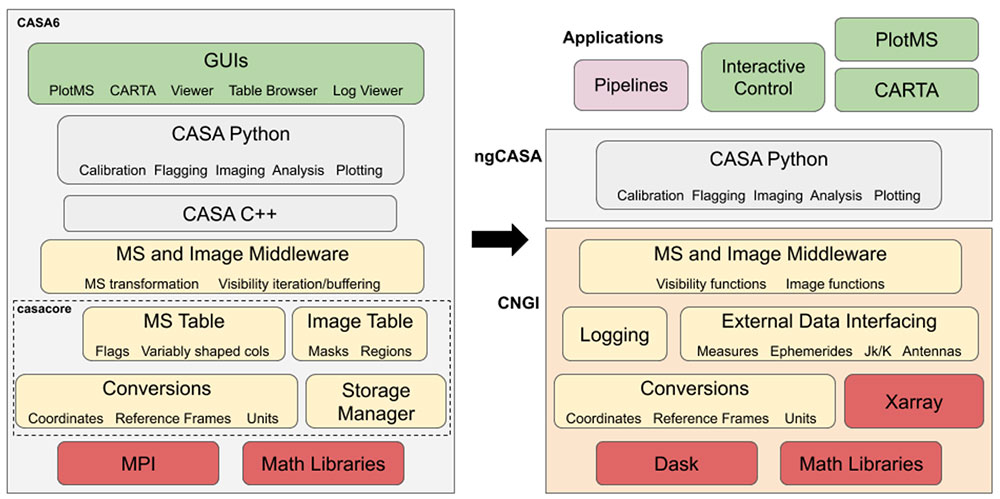
The CASA team is now in the early stages of design for the next generation of CASA (ngCASA), beginning with a CASA Next Generation Infrastructure (CNGI). CNGI will provide a replacement to the infrastructure and middleware layers of CASA using largely off-the-shelf products that are dramatically simpler to use and scalable to a variety of large computing environments. After two rigorous trade studies, the Xarray Dataset and Dask parallel processing framework were selected as the foundation for new data structures and scalable processing in the Python language.
The CNGI package will include new implementations of MeasurementSet and Image data manipulation routines found in casacore and middleware layers of CASA today, but realized in an entirely new paradigm.
The core CASA science functionality of flagging, calibration, imaging and analysis will be rebuilt atop the new CNGI infrastructure. The design of this ngCASA layer is still taking shape, but is intended to follow a functional approach, with Xarray dataset objects passed in and returned by stateless ngCASA / CNGI Python functions. This isolates all software state, processing, and file I/O in the Xarray objects which in turn is handled by the Dask engine, dramatically simplifying the code complexity of CASA itself.
A final “Application” layer will be created above ngCASA to separate use cases and user bases with more appropriate and specialized interfaces. This allows for better separation of such things as manual interactive users from headless automated pipelines, and allows ngCASA functions to develop in a way that makes better technical sense.
CNGI prototyping using Dask and Xarray is currently underway, with the new design starting to take shape, new structures created for holding visibility (MS) and image data, and a range of new preliminary functions starting to be populated. Further details and a Python pip-installable prototype package can be found here.
The prototyping effort has placed heavy emphasis on performance and scalability, with the goal of servicing next generation instruments such as ngVLA and SKA. Benchmarking is ongoing as new capabilities are developed, but early indications from imaging functionality developed so far suggest significant gains for larger than memory dirty image creation (gridding and fast Fourier transform).
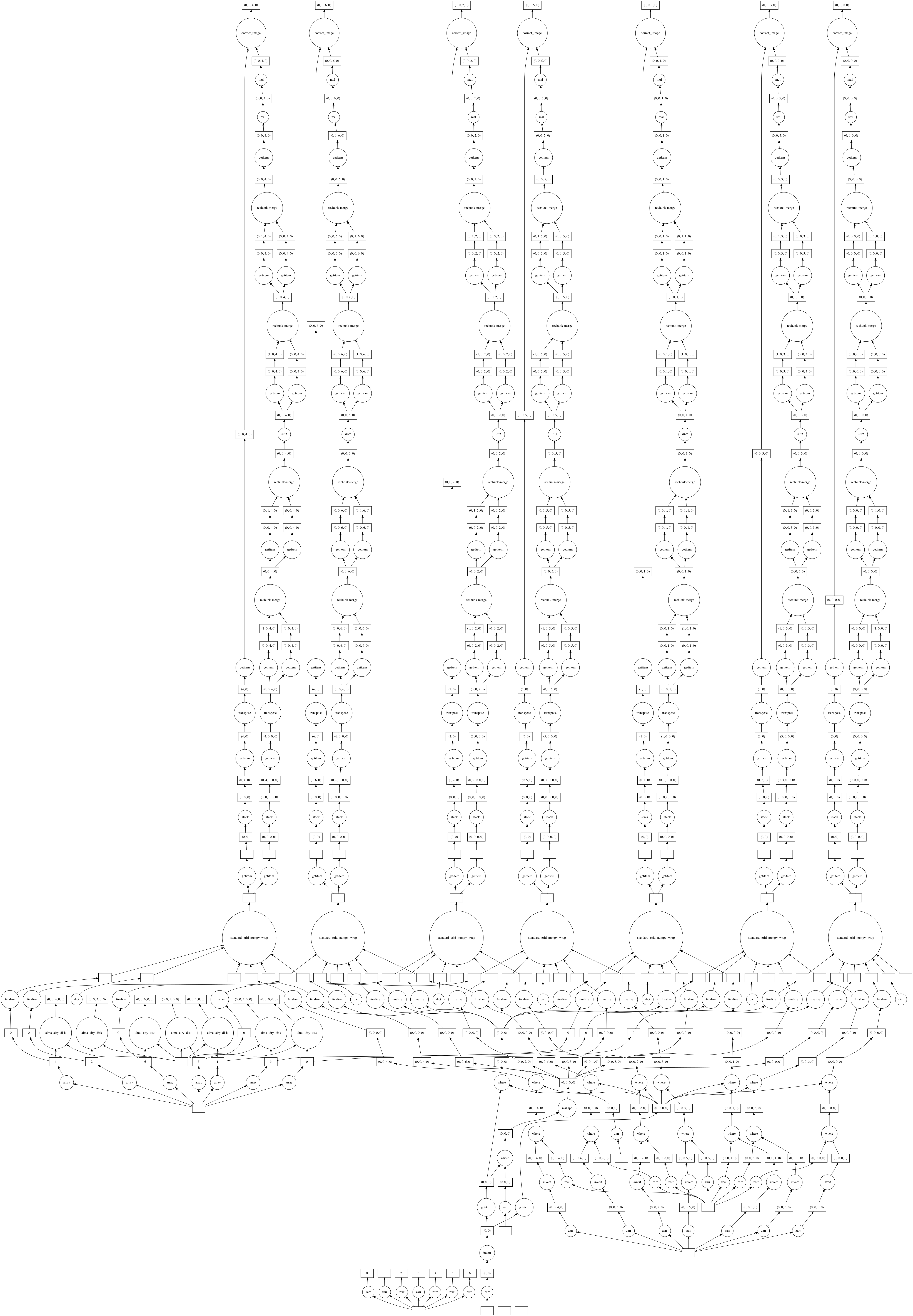
ngCASA operations build up a directed acyclic graph (DAG) in CNGI. The DAG sequence is processed together for increased efficiency over the traditional method of executing each operation one at a time in isolation. This DAG creates a cube image with data that has seven channel chunks.
The VLA Sky Survey Single Epoch Images
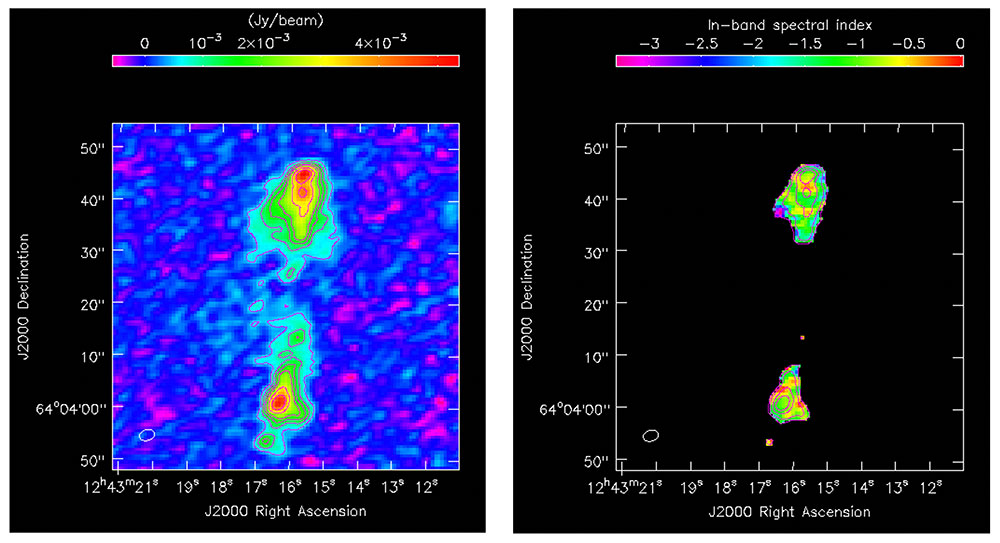
An FRII radio galaxy from on one of the VIP test images. [Left] Total intensity. [Right] In-band spectral index image (masked at a continuum signal-to-noise of 10-sigma per beam).
[click to enlarge]
The VLA Sky Survey (VLASS) has been imaging the entire radio sky visible to the VLA in S-band, B-configuration since September 2017. VLASS observations cover half the sky each time the VLA is in B/BnA-configuration, and last summer we completed the first of three planned passes over the sky.
Immediately after observation the data are calibrated and then imaged using the “Quick Look” (QL) imaging pipeline. This pipeline uses the mosaic gridder in CASA to produce Stokes I images. The use of the mosaic gridder means that images can be produced quickly, as soon as a few days after observation, important for those studying transient sources. The accuracy of these images is, however, limited by the neglect of the non-coplanar baselines in the mosaic gridder. In particular, a position distortion dependent on the zenith distance of the observation is introduced that typically ranges between 0.2-1 arcseconds. The PSF is also affected, limiting the dynamic range and flux density accuracy of the images. The positions can be improved to within ~0.2 arcseconds by applying a correction to the central position of each 1 deg2 VLASS image (these corrections are applied to the VLASS 2.1 QL images, and will be applied retroactively to VLASS 1.1 and 1.2), but the other non-coplanar effects remain. For the final images for each VLASS epoch–the so-called Single Epoch (SE)–images (which also include spectral index information missing from the QL images), a more accurate algorithm was therefore needed.
The aw-project gridder in CASA correctly accounts for the non-coplanar terms, and experiments indicated that this could offer the required accuracy, but at the expense of a much larger computational load and additional problems with convergence of the clean algorithm. To tackle the convergence issues, and to come up with a recipe for making the SE images that included self-calibration (that had been missing from the QL images) the VLASS Imaging Project (VIP) was started in January 2020 and ran for three months. Convergence issues were addressed by using an initial clean mask based on component identification from the QL image cleaned with a uniform-weighted image, both for model creation and to identify additional source components not present in the initial clean mask. Final images were then creating using a standard Briggs robust=1 beam. The end result of this project (detailed in VLASS Memo #15) was an improved set of test images satisfying the survey requirements for positional and flux density accuracy, RMS noise, and dynamic range.
The computational challenge remained though. Each 1 deg2 test image took ~ 1 week to make on the NRAO cluster, and, although several can be run in parallel, it would still take many years to image all 34,000 deg2 using NRAO facilities alone. To tackle this problem, NRAO is adopting a High Throughput Computing (HTC) approach in collaboration with the Center for High Throughput Computing at the University of Wisconsin-Madison. HTC is distinct from High Performance Computing (HPC) in that HTC emphasizes throughput of jobs rather than speed, and it is throughput that is needed in our case.
The first step is to make the imaging jobs more amenable to current HTC platforms. This involves reducing the memory footprint of the imaging jobs to better suit the small memory but large number of cores on a typical HTC cluster node. To achieve this, the imaging is split into subtasks, operating on subsets of the Measurement Set being imaged. The imaging job is thus split into many smaller jobs, with the results being gathered together at the end of the process. The details of this workflow are currently being finalized, but initial tests are promising. With this new workflow in place and the extra resources that we will be able to take advantage of by using it (for example, the Open Science Grid) we expect to be able to hit our target of imaging 1000 deg2 per month, which will allow us to keep pace with the observations for the second and third epochs of VLASS. The next step will be to adapt these algorithms to make the Stokes I, Q and U cubes intended for polarimetric studies.
CARTA v.1.4 Release
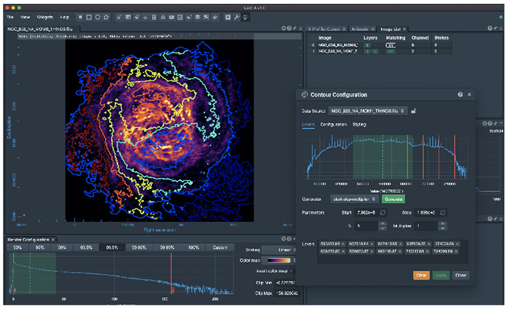
Overview of the CARTA Visualization Software
[click to enlarge]
CARTA v. 1.4 has been released and is now available from the redesigned homepage. The Cube Analysis and Rendering Tool for Astronomy has streamlined features that are crucial for the visualization of astronomical data cubes. As with earlier versions, CARTA is designed for performance with substantial decreased loading times for large images and cubes compared to other visualization programs. The v1.4 is now ready for visualization of multiple datasets with world coordinate and spectral alignments (see the image for an example of a THINGS data set). In addition, new features were added to CARTA, including:
- Catalogue support
- Shared region analytics
- Animation playback improvement of raster and contour images
- Profile smoothing
- Moment map generator
- Spectral line query
- Server authentication and deployment improvements
- File browser improvements
- Bug fixes and performance improvements.
These features are on the path to add the full analytics that are currently included in the CASA viewer. In addition, new options, like the catalogue overlay support, add additional functionality that are not present in the CASA viewer. We encourage all CASA users to start making the switch from the unsupported CASA viewer to CARTA for all image viewing capabilities currently supported in CARTA.
A roadmap for upcoming features is provided on the CARTA webpage. For questions and suggestions, please contact the CARTA team.Single Dish
Spectral Imaging of Moving Sources
CASA now completely supports single-dish spectral imaging of moving sources. Moving sources, such as near field objects or solar system objects, can be tracked along the frequency axis as well with CASA 5.7/6.1 or later, in addition to tracking their celestial position on the sky that has been already available in the earlier releases.
The task tsdimaging, to make image cubes of single-dish data, has a new option ‘cubesource' for the parameter specmode now. Setting specmode='cubesource' as well as specifying ephemeris table name or 'TRACKFIELD' for the phasecenter parameter, the systemic radial velocity of the source is accounted for so that the frequency reported will be in the rest frame of the source.
Using this capability, users can finally see the correct frequency or velocity structure of emission lines for moving objects, which gives insight into their physical status and/or motion.
Revised Release Schedule for the Nobeyama Pipeline (NRO Pipeline)
In the previous newsletter (CASA Newsletter Issue 9), we indicated that we planned the initial release of the NRO Pipeline in late 2019. However, this schedule was found to conflict with the important activity of the pipeline development team to port the pipeline code to Python 3. Given the limited lifetime of releases based on Python 2.7, which will soon be obsolete when porting to Python 3 is complete, we decided to reschedule the initial release and make it compatible with Python 3. The revised schedule is to release the Pipeline for both ALMA and Nobeyama in October 2020. We believe that the decision benefits both users and developers.
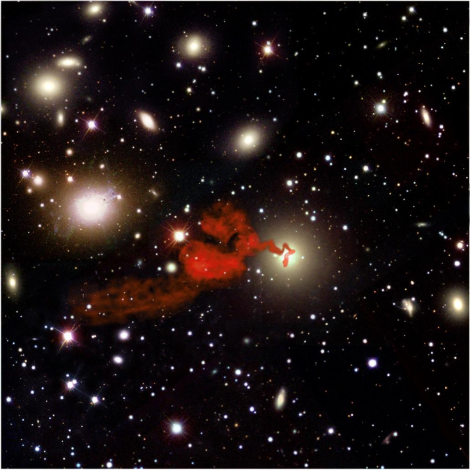
Stunning Views of the Cosmos: NRAO Image Contest
In celebration of the 40th anniversary of the Karl G. Jansky Very Large Array (VLA), held on 10 October 2020, astronomers from around the world joined NRAO’s VLA image contest. Entries displayed a compelling range of celestial phenomena, beautifully illustrated by our user community. The end result is a series of images with high visual impact, making them compelling for public audiences as well as the scientific community.
The winning entries, and those earning honorable mentions, relied heavily on the CASA software to turn the raw VLA data into these stunning visualizations. CASA’s advanced algorithms for imaging and calibration, such as awprojection and polarization calibration, were instrumental in giving us these unique new views on the Universe.
The CASA team would like to congratulate the winning teams with these inspiring results!
The first prize winner, Giannandrea Inchingolo of the University of Bologna, showcases a video that displays a collision of cluster of galaxies, made by combining VLA radio observations with computer simulations.
The second prize winner, Jayanne English of the University of Manitoba, made a beautiful composite VLA and Hubble Space Telescope image that reveals the extended magnetic field of galaxy NGC 5775.
The third prize winners, Marie-Lou Gendron-Marsolais and Chat Hull, both residing in Santiago with ESO/ALMA and NOAJ, combined VLA data with color-imaging from the Sloan Digital Sky Survey to showcase enormous jets emanating from the giant galaxy NGC 1272 in the Perseus Cluster.
More information can be found in an NRAO press release.
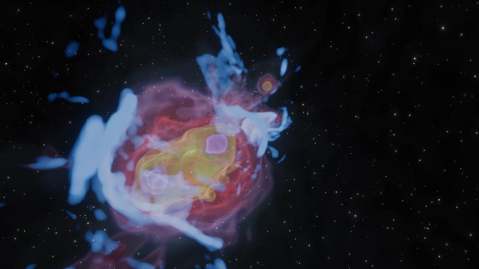 |
First Prize: Radio Relics in Galaxy Clusters – Collisions – Simulations & VLA |
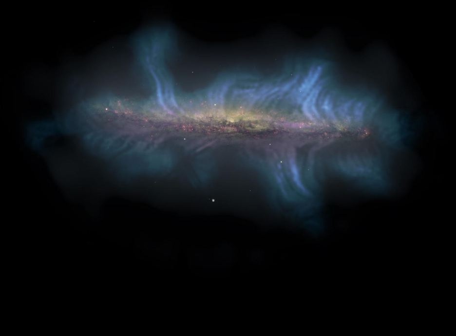 |
Second Prize: Magnetic Field in Galaxy NGC 5775 – HST/VLA. |
 |
Third Prize: NGC 1272 jets in Perseus Cluster – Sloan/VLA |
Credits
First Prize: Radio Relics in Galaxy Clusters – Collisions – Simulations & VLA
Scientific data by D. Wittor (University of Hamburg – simulation), C. Stuardi, K. Rajpurohit (University of Bologna – VLA observation).Video realized by G. Inchingolo, P. Zuzolo (University of Bologna), S. Imboden D. De Luca (CINECA Visit Lab). Audio realized by sonification of the simulation data used for the video by J. Paradiso (MIT Media Lab)
Second Prize: Magnetic Field in Galaxy NGC 5775 – HST/VLA
Composite image by Jayanne English (University of Manitoba). NRAO VLA data processed by Yelena Stein (CDS) for the Continuum HAlos in Nearby Galaxies — an EVLA Survey (CHANG-ES) led by Judith Irwin (Queen’s University, Canada). The optical data are from the Hubble Space Telescope (HST) Wide Field Camera 3 (WFC3). The software code for tracing the magnetic field lines was adapted by Y. Stein, J. English and Arpad Miskolczi (Ruhr-University Bochum) from the scipy Line Integral Convolution code (https://scipy-cookbook.readthedocs.io/items/LineIntegralConvolution.html).
Third Prize: NGC 1272 jets in Perseus Cluster – Sloan/VLA
Sloan Digital Sky Survey (filters: colored in blue, green and red), VLA, M. Gendron-Marsolais, C. L. H. Hull.
Issues Concerning Ionospheric Calibration File Retrieval and Processing
In CASA, support for ionospheric calibration (dispersive delay and Faraday rotation, especially at longer wavelengths) is aided by use of a helper script distributed with the package: tec_maps.py. This script, originally contributed to CASA by Jason Kooi while a graduate student at the University of Iowa (now at NRL), implements retrieval of total electron content (TEC) files from NASA's Crustal Dynamics Data Information System (CDDIS), and from them forms TEC surface images that can be supplied to the CASA gencal task to generate an ionospheric calibration table. Use of the tec_maps.py script is described in the online CASA Calibration documentation.
At this time, there are temporary issues that interested users should be aware of. First, the tec_maps.py script has not yet been ported to python3-aware CASA 6.x. This effectively means that ionospheric calibration is not supported in CASA 6.0 or 6.1, although TEC surface images generated by any CASA 5.x installation will be usable in gencal in CASA 6.x. The tec_maps.py script will be made python3-compliant for the CASA 5.8/6.2 release expected in late 2020.
Second, the NASA CDDIS has recently revised its services to introduce a greater degree of security, and the traditional retrieval mechanism (anonymous ftp) will be disabled as of 31 Oct 2020. Unfortunately, the CASA 5.7 release in August 2020 did not include the necessary updates to its CDDIS retrieval call, and so tec_maps.py's internal file retrieval will break at the end of October. At that point, it will become necessary for users to manually retrieve the required TEC file(s). The existing tec_maps.py script will then use these files instead of attempting the retrieval.
For each UTC day spanned by your dataset, the manual file retrieval can be accomplished outside CASA as follows (each command all on one line):
$ curl -u anonymous:<your-email-address> --ftp-ssl ftp://gdc.cddis.eosdis.nasa.gov/gps/products/ionex/YYYY/DDD/igsgDDD0.YYi.Z > igsgDDD0.YYi.Z
$ uncompress igsgDDD0.YYi.Z
The filename convention corresponding to the observation date is as follows: YYYY is the full year number (e.g., 2020), DDD is the 3-digit day number within the year, and YY is the 2-digit year number (e.g., 20). Don't forget to uncompress the retrieved file(s)!
As written above, this command will attempt to retrieve the "IGS Final Product" file, which typically is not available for as much as 12-14 days following the date of observation. If provisional (and presumably less accurate) TEC information is desired sooner, substitute 'igsg' (in both places) with 'igrg' or 'jprg', to attempt retrieval of, respectively, the "ISG Rapid Product" (available 2-3 days post-observation) or "JPL Rapid Product" (available 1 day post-observation) file.
Execution of the tec_maps.create0 function in CASA will then opt out of the retrieval call and instead use these files to generate the TEC surface map if they are present in your working directory.
The tec_maps.py script will be updated with the revised retrieval call in the CASA 5.8/6.2 release, expected in late 2020.
More detailed information about the retrieval protocol changes on the CDDIS server can be found online, where several alternative retrieval mechanisms are also described.
Users having problems with this interim mechanism for TEC retrieval should submit a request for help to the NRAO Helpdesk.
