
CASA News
Issue 2
19 October 2015

CASA News
Issue 2 • 19 October 2015

Letter from the Lead
As summer turns to autumn in New Mexico, we are putting the final touches on the CASA 4.5 release. CASA 4.5 delivers several long-running projects, a refactored clean, scratch-less application of calibration tables in plotMS, and the parallelization framework. We are moving forward toward the next release, focusing on improving reliability and robustness throughout the system.
The data reduction workshops held at NRAO were rated highly in the CASA User Survey in terms of usefulness. Watch for an announcements of the upcoming reduction workshops for ALMA and the VLA – January and March 2016, respectively – in the NRAO eNews. We recently received a suggestion that a workshop for advanced users dedicated to a more detailed discussion of CASA’s finer points would be very useful. NRAO is in the beginning stages of designing such a workshop and would like your input. A brief on-line survey is now available that is designed to gather input regarding which topics are of greatest interest to the user community.
Finally a word on operating systems planning. In accord with our policy of supporting the two latest versions of the OSX operating system, we are planning to release an OSX 10.11 version of CASA 4.6 next spring. At that point, we will discontinue support for OSX 10.9. On the Linux side, we will continue to support RHEL 5 and 6 for the CASA 4.6 release, and will assess adding support for RHEL 7 and discontinuing RHEL 5 support for the following release.
CASA User Survey Results
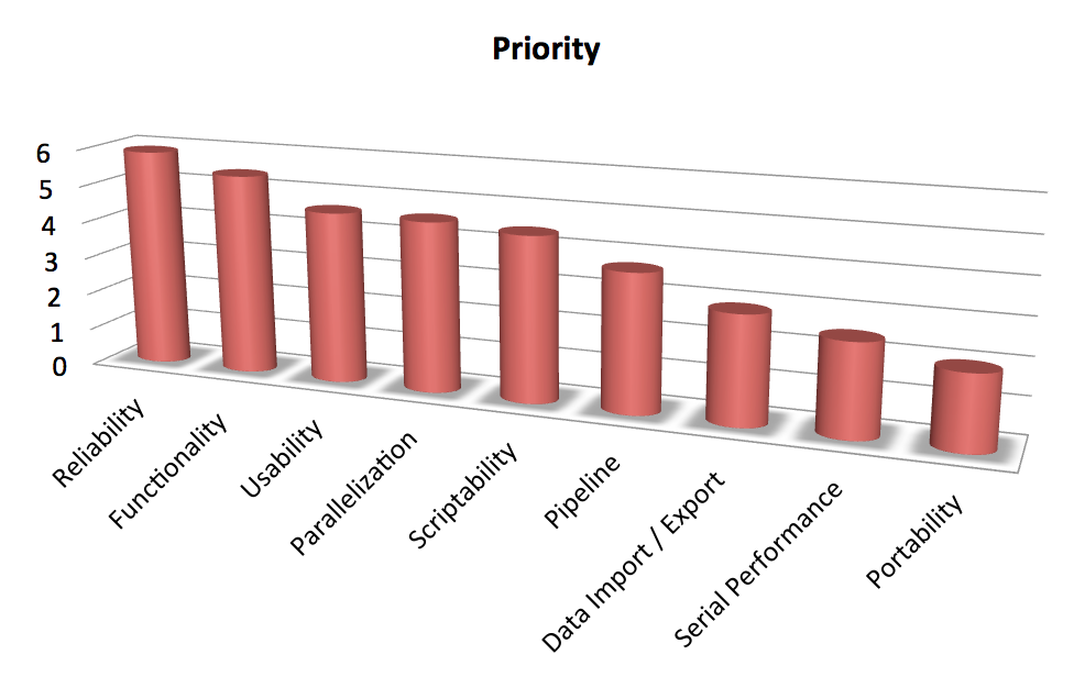
Development priority determined from CASA User Survey. Improving the reliability of CASA is ranked as most important.
[click to enlarge]
Thank you to everyone who participated in the CASA User Survey. The survey was executed 6-22 March 2015, and a total of 252 responses were recorded. We appreciate your taking the time to provide feedback about your CASA use and concerns. We have carefully analyzed the responses and are incorporating your input into our development and planning.
Demographics
Good representation from all career stages – 16% graduate student, 26% postdoctoral fellow, and
36% faculty or Research position – is present in the sample as well as different institutional settings: 43% of the respondents are in a university environment, while 26% and 13% are in observatory and national labs, respectively. Nearly all participants ranked themselves as intermediate or expert in radio astronomy: less than 5% ranked themselves as beginner or no experience.
As might be expected for a CASA User Survey, CASA is the most frequently used data processing package. The AIPS and MIRIAD packages are used rarely by the respondents, with a smattering of use of other packages. Most respondents frequently use CASA. A significant number of users (30%) use CASA every day; surprisingly, this number increases if you exclude observatory users.
Documentation & Communication
The need for clear, consistent, and up-to-date descriptions of the CASA implementation was a major theme in the responses. We are working with the CASA Users Committee to design and curate a less static and more informative documentation approach. One of the survey questions assessed the frequency and usefulness of our documentation. From the responses, it is clear that the CASA guides are widely used and highly useful. We will work with the scientific support groups to maintain and improve these. The Cookbook and inline help are also frequently used but considered less useful. Improving the coordination and usefulness of these references is an issue that we are working to address.
NRAO data reduction workshops scored quite highly in terms of usefulness but have limited participation. The expert community found these somewhat less useful. We are considering an Expert Data Reduction workshop aimed at more advanced users. We welcome your input on how we should structure such a workshop and have created a brief survey to collect your suggestions.
Hardware
A large section of the survey asked about the computing platforms used to process data. It was intended that the survey provide information about workstation systems and a separate set of questions about other systems, such as laptops. Unfortunately, the question wording was insufficiently clear and the results reflect this confusion. We can say, however, that most CASA processing is taking place on multi-core systems with ~4 GB of RAM per core.
Single hard-drive systems account for approximately half of the systems described in the survey. For a modern multi-core system, the implication is that trading additional computation for decreased I/O operations should improve the users experienced performance. We have already been moving in this direction as, for example, in the creation of the virtual model column, and the on-the-fly application of calibration in plotMS.
CASA is being used on a wide range of operating systems and versions. Although OSX represents nearly half of the monthly CASA downloads, it represents only a quarter of the overall usage. Various forms of Linux represent the majority of the usage, with Ubuntu the most commonly installed (30%).
Development Priorities
The survey requested respondents provide input on nine broad categories of development and rank them in priority order. The top priority per the survey is increased reliability, followed by increased functionality. This input is consistent with the guidance of the CASA Users Committee and the NRAO Users Committee. We are working to complete the on-going functionality initiatives but are turning our attention to improving the quality and reliability of the software. Improving test coverage, removal of obsolete and confusing tools, and improved documentation are all high priority tasks for the development team.
Usability, parallelization, and script-ability are all given approximately the same ranking and are the third tier of priorities. The remaining priorities were pipeline development, data import/export, serial performance, and finally support of other OSs. Although we do not plan to eliminate any of these efforts, this clear community prioritization will be key inputs as we prioritize development in the upcoming cycles.
Features and Comments
The final two survey questions provided an opportunity for general comments and features.
Three topics stood out as most frequent in these comments.
Documentation: As described above, accessible, current, and concise documentation is a frequent request, and we are working on a plan to improve the CASA documentation.
Very Long Baseline Interferometry (VLBI): Support for VLBI and, in particular, fringe fitting was a frequent request. The CASA team is working to develop collaborations to address this missing functionality.
Viewer: The shortcomings of the CASA viewer were often noted. In the ALMA development program, CASA is part of the University of Alberta-led CARTA project to implement a next generation cube viewer. This is intended replacement for the CASA viewer once it has completed the initial development cycle.
Final Notes
“Thank you” again to everyone who completed this survey. The CASA team plans to periodically conduct similar surveys which will be announced in the CASA News.
CASA Image Processing
[click to enlarge]
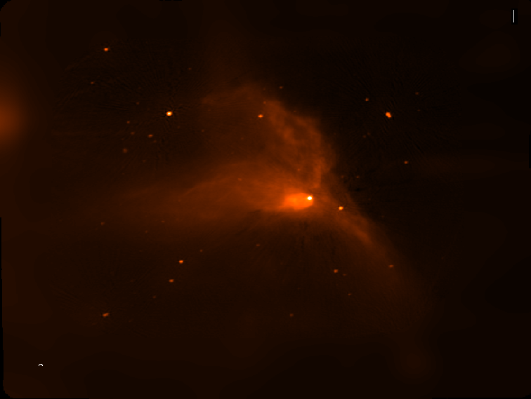
This preliminary wide-band mosaic in Stokes-I of a ~2 x 2 degree region in the Galactic Plane combines wide-band, L-band data from the Very Large Array (VLA) and the Green Bank Telescope (GBT) and was observed with 100 VLA pointings and GBT raster scanning. Data flagging and calibration were done semi-automatically; one field was affected by an artificial satellite pass through the beam and required manual flagging. VLA imaging was accomplished using parallel processing via the new tclean interface to the CASA Imager module. Using 106 cores for processing on ~250GB of calibrated data, WB AW-Projection algorithm for imaging, and MT-MFS algorithm with 2 Taylor terms and 3 scales for deconvolution, creating this image required ~10 hours run time, including some wait-time for manual masking. The GBT data were combined using the CASA feathering algorithm. Further work is underway to enable spectrally combining GBT and VLA data, as well as to further improve spectral index (not shown here) and full-Stokes mapping.
Credits
Imaging: S. Bhatnagar, U. Rau & A. Roshi (GBT data)
Pilot Survey: S. Bhatnagar (NRAO), U. Rau (NRAO), M. Rupen (DRAO), K. Golap (NRAO), D.A. Green (Cambridge, UK), R. Kothes (DRAO), A. Roshi (NRAO), S.M. Dougherty (DRAO), P. Palmer (Chicago)
News from the Helpdesk
Over the past six months, we have received 247 tickets through our Helpdesk system, supporting CASA processing of VLA, ALMA, and other telescope data. Questions have come in from users asking how to combine data from different ALMA data sets. Recent changes in the way CASA calculates visibility weights require a careful approach to data combination. In response to these questions, an in-depth CASA Guide has been published that explains the data combination process. Please review the guide and contact us via the ALMA Helpdesk if you have additional questions.
We have also recently seen Helpdesk tickets about errors encountered when updating the data repositories – geodetic information, leap seconds, ephemerides, flux models, etc. – distributed with CASA. CASA sends warnings when the leap second table is about six months old, which should only affect few users. The repository can be updated using the command !update-data inside CASA. However, some recent changes to the way these tables are distributed has resulted in rsync errors. To fix this problem for CASA 4.4 or earlier, we have created a patch that can be run from the terminal:
$ update-data.patch <PATH-TO-CASA-DISTRIBUTION>
<PATH-TO-CASA-DISTRIBUTION> is the path to the top level of the unpacked CASA distribution. A KnowledgeBase article is also available to assist with this issue.
As always, we are glad to hear from you. So, keep the Helpdesk questions coming!
Ephemerides in CASA
Support for the analysis of interferometric or single-dish observations of ephemeris objects has been available for some time and a well-tested workflow version was offered in CASA 4.4. This involved attaching a user-provided, JPL-Horizons ephemeris to an arbitrary field of an MS using the task fixplanets and later using the task cvel to perform the spectral reference frame transformation to the object's rest frame. Details are described in the CASA Cookbook.
With CASA 4.5, the support for ephemeris objects in ALMA data has taken another large step towards completion. Now it is possible to obtain the ephemeris used during the observation integrated in the ALMA raw dataset or Science Data Model (SDM). Upon import to MS format, the ephemeris is automatically attached to the corresponding field(s) and used whenever the direction of the object is needed. For the spectral frame transformation, however, the user still needs to run cvel or, as a faster alternative, the new task mstransform. This article describes this process in more detail.
Beginning with Cycle 3, the ALMA observatory will include in each SDM all necessary ephemerides in the so-called Ephemeris table, an XML file inside the SDM. Each ephemeris in the table has a separate ID. The task importasdm will translate each of these ephemerides into a separate CASA ephemeris table which has the same format as those used by the task setjy. Examples can be found in the subdirectory "data/ephemerides/JPL-Horizons" in each CASA distribution. The task importasdm will then automatically attach these CASA ephemeris tables to the fields they belong to such that they are ready for use when importasdm is completed.
The ephemerides used by ALMA are originally for the observer location of ALMA. They use the ICRS coordinate reference frame and typically have a time spacing of a few tens of minutes. For the later transformation of the spectral reference frame, however, a geocentric ephemeris is preferable and presently required. The importasdm task will therefore by default also perform a conversion from the ALMA observer location to the geocenter. This is controlled by the new importasdm parameter "convert_ephem2geo" which is True by default.
The spectral reference frame of the visibilities in the SDM is always topocentric (TOPO), the observer reference frame. For the observation of lines in the rest frame of the ephemeris object, it is necessary to transform the visibilities to that frame. This software Doppler tracking can be achieved with either the traditional task cvel or its new, faster implementation cvel2 which uses internally the same code as the new task mstransform. All three tasks produce the same result.
As described in the CASA Cookbook, the user must set the "outframe" parameter of cvel, cvel2, or mstransform to "SOURCE". This will lead to a transformation from the TOPO to the GEO reference frame followed by an additional time-dependent Doppler correction according to the radial velocity of the object as given by its ephemeris.
When an ephemeris is attached to a field of the MS FIELD table, the object position is no longer taken from the direction columns of the FIELD table but linearly interpolated from the ephemeris table for the given time. The nominal entry of the direction column then changes its meaning to an angular offset with respect to the ephemeris. Thus, if the object is exactly at the position described by the ephemeris, the nominal entries of the direction column are zero for right ascension and declination. If, e.g. in the case of a mosaic, there are a number of fields with nearby positions, the fields can share an ephemeris; they all reference the same ephemeris table via the optional column EPHEMERIS_ID, but have in their direction column entries different offsets.
Because the user can no longer expect that the nominal field direction entries are the actual object position, it is now (since CASA 4.3) necessary to obtain the field direction with special tool methods
msmd.phasecenter()
or the more general
ms.getfielddirmeas()
(see the built-in CASA help for details). The default time of the position is taken from the TIME column of the FIELD table.
In summary, with the new way of delivering ephemerides included in the ALMA raw data and the added support for this in the importasdm CASA 4.5 task, the user will no longer have to worry about how to obtain the right ephemeris in the right format and how to attach it properly to the MS. This process will now be entirely transparent and only a few additional logger messages will indicate that this is happening. The correct time-dependent positions, radial velocities, and object distances will then
be used in all relevant tasks such as listobs, plotms, and, as described above, cvel, cvel2, and mstransform. For Solar-System object flux calibrators, the task setjy will, however, only extract the nominal position from the SDM ephemeris and otherwise use its internal set of ephemerides since these contain additionally needed object parameters. Care has to be taken when trying to extract the field positions from the FIELD table as the nominal direction column entries will only be offsets if an ephemeris is attached.
Similar support is also in preparation for ephemerides in VLA data that use a polynomial representation of the positions and radial velocities rather than the tabulation approach of ALMA. Completion of this support is expected for CASA 4.7 at the latest.
Parallel Processing in CASA
Starting in CASA 4.5.0, an execution of a full data analysis from data import to imaging is possible using a new infrastructure based on the Message Passing Interface (MPI). Not all the steps in the data analysis are ready to be used in parallel. For example, parallel use of tclean is still undergoing internal testing and is not yet recommended for routine use. On the other hand, importing, calibration, flagging, averaging and splitting are parallelized.
The parallelization in CASA is achieved by partitioning the MeasurementSet (MS) of interest using the task partition or at import time using importasdm. The resulting partitioned MS is called a Multi-MS or MMS. Logically, an MMS has the same structure as an MS but internally it is a group of several MSs which are virtually concatenated. Each member MS or Sub-MS of an MMS, however, is at the same time a valid MS on its own and can be processed as such.
Once the data is partitioned in a Multi-MS, the CASA parallelized tasks are able to detect it automatically and if a cluster is available, sub-tasks are sent to the cluster nodes over MPI. Once all sub-tasks are completed, the results are consolidated before returning to the user. To run in cluster mode, the CASA distribution comes with a custom MPI launcher called mpicasa, which properly configure the environment to run CASA in parallel.
The following is a typical example on how to run CASA in parallel using mpicasa and a parallelized script on a multi-core desktop:
mpicasa -n 5 casa -c alma-m100-analysis-hpc-regression.py
The above example will use five cores of the local host, where four cores will run an instance of CASA in parallel to process a separate Sub-MS. The first core will be used for cluster management and interaction with the user. The alma-m100-analysis-hpc-regression.py script already contains a call to importasdm that creates a Multi-MS so that the processing can happen in parallel.
The parallelization in CASA is available for Linux systems only. The user should be aware that running CASA in parallel on a NFS mounted system will likely not yield the desired gain performance. The ideal requirement is a common high-performance file system for multi-node use and a strong I/O system.
The performance gain will depend on several items, in additions to the above mentioned requirement.
- The type of processing done in the analysis. For example, if the processing makes large use of the parallelized tasks, the processing will be faster.
- The size of the ASDM in order to decide if it is worth processing in parallel or not.
- In the ideal case, there should be one processing core per Sub-MS, but there is a maximum limit in the number of Sub-MSs to create, which depends on the spw/scan content of the MS.
The following tasks are parallelized, which means, they will run in parallel on each of the Sub-MSs of the input MMS:
|
|
Our tests show a speed increase of 1.55x when running the alma-m100-analysis-hpc-regression.py script (without the imaging steps) in parallel. The test was performed with five cores in a system with read/write limit of 150 MB/s.
See the latest CASA 4.5 Cookbook for a full explanation on how to create a MMS and run CASA using MPI.
On-the-Fly Calibration in Plotms
As of CASA version 4.4, users can view calibrated data in plotms without first running applycal. Using a new "callib" parameter in the plotms task, a calibration library file containing calibration application instructions can be set. The corrected data is produced on the fly and displayed in the plot. For example, consider a MeasurementSet, ngc5921.ms, and a plot of the observed visibility amplitudes versus frequency generated by the following command:
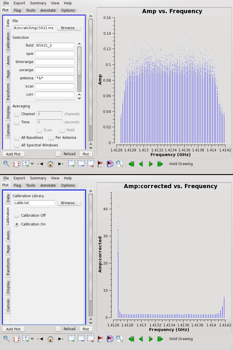
Fig. 1: The NGC 5921 MeasurementSet without the calibration applied (above), and with the calibration applied (below).
[click to enlarge]
plotms(vis='ngc5921.ms', xaxis='frequency',

  yaxis='amp', ydatacolumn='data',  # request observed amplitudes

  field='N5921_2',                  # an HI galaxy

  antenna='*&*')                    # avoid auto-correlations
To view these data calibrated with a calibration library file called 'callib.txt', use this command:
plotms(vis='ngc5921.ms', xaxis='frequency',

  yaxis='amp', ydatacolumn='corrected',  # request corrected amp

  field='N5921_2',                       # an HI galaxy

  antenna='*&*',                         # avoid auto-correlations

  callib='callib.txt')                   # enable OTF calibration
The data will appear as in Figure-1 with and without the calibration.
Calibration is enabled ("Calibration On") when the callib parameter is set and its contents validated. The 'corrected' must be explicitly requested in the “ydatacolumn” or “xdatacolumn” parameter to be seen in the plot. Use of the “callib” parameter merely enables on-the-fly generation of calibrated data, if it is requested for the plot. Other options for “ydatacolumn/xdatacolumn” remain operational and will behave as expected.
From the GUI, a calibration library file can be selected using the file browser in the new Calibration tab. Calibration is enabled or disabled using the Calibration On/Calibration Off radio buttons. When these selections change, the text is shown in red and the user must click the Plot button to see the results. If calibration is disabled and corrected data is requested, the existing corrected data column in the Measurement Set is displayed. If this column does not exist, the uncorrected visibility data is displayed with a log warning: "CORRECTED_DATA column not present and calibration library not set or enabled; will use DATA instead."
The calibration library file allows the user to specify calibration instructions per Measurement Set selection for multiple caltables, consolidating the process into a single execution. The 'callib.txt' file used above contains the following lines:
caltable='ngc5921.bcal' calwt=True tinterp='nearest'
caltable='ngc5921.fluxscale' calwt=True tinterp='nearest' fldmap='nearest'
# comment allowed in callib file
caltable='ngc5921.gcal' calwt=True field='0' tinterp='nearest' fldmap=[0]
caltable='ngc5921.gcal' calwt=True field='1,2' tinterp='linear' fldmap=[0,1,1,3]
Further documentation on the calibration library syntax can be found in Appendix G of the CASA Cookbook.
CASA-based Pipelines
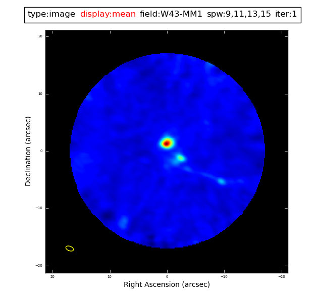
ALMA Band 6 continuum image of W43-M1. Produced by the ALMA imaging pipeline. Data provided courtesy of P. Cortes et al.
[click to enlarge]
The period following publication of the debut CASA News has been a busy one for the pipeline team. The focus of the ALMA interferometry pipeline development shifted from calibration and flagging to imaging and providing support for High Performance Computing (HPC) enabled CASA; the VLA calibration pipeline transitioned to operational status; and the ALMA single dish pipeline achieved a recommendation for full acceptance.
Early in 2015, ALMA Science Operations drafted a document defining the standard interferometry image products. The image product list includes: a per science target, per receiver band combined spw continuum map; a per science target, per spectral window, full resolution frequency cube; and a per science target, per spectral window frequency cube at the user specified resolution, if this resolution is significantly different from the native resolution. The pipeline imaging recipes required to produce these products have been implemented. They are constructed around the new HPC-enabled CASA tclean task and a sophisticated spectral feature finding algorithm developed by the North American ALMA Science Center (NAASC) staff. At the time of writing, the pipeline team is preparing an internal pipeline release containing the new imaging recipe for testing and validation by the Pipeline Working Group.
Work continued on improvements to the ALMA interferometry calibration pipeline heuristics. The January 2015 pipeline release, which includes low signal-to-noise ratio (SNR) bandpass and phase calibration narrow to broad spectral window mapping heuristics, was released to the user community as an add-on to CASA 4.3.1. Work on additional long baseline, low SNR calibration heuristics is in progress.
Using Cycle 1 and 2 data, ALMA Science Operations compared the effectiveness of the pipeline flagging heuristics to the manual flagging procedures. Two areas for pipeline improvement were identified: (a) propagate the ALMA QA0 process flags to the ASDM(s) so that the pipeline can make use of them; and (b) implement a new per antenna outlier amplitude versus time-flagging heuristic to complement the current anomalous gain detection heuristics. Pipeline support for QA0 flagging will available in the next pipeline release. The outlier amplitude versus time algorithm is under development.
The VLA calibration pipeline is in routine operation. This pipeline is triggered automatically by the arrival of completed data sets in the VLA archive. Plans for improvement include implementing low SNR heuristics to improve the calibration, implementing support for polarization calibration, and evaluating the requirements for generating science target image data products and supporting the VLA Sky Survey.
The ALMA single dish pipeline achieved recommendation for full acceptance in September. A great deal of effort by the ALMA single dish team was spent over the past several months, acquiring representative test data, running the pipeline in parallel with manual reductions, comparing the results, improving the web log, and improving runtime efficiency.
Future pipeline work will focus on pipeline HPC operations, accessing catalog information where appropriate, and supporting new observing modes.
Imager Refactor
[click to enlarge]
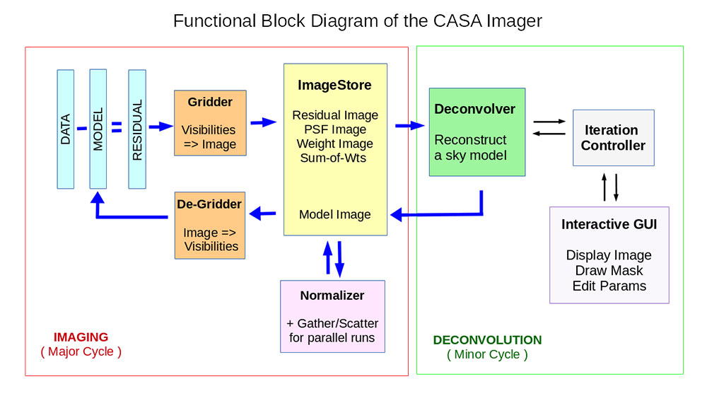
We have been rewriting the application layer of the CASA Imager. Core gridding and deconvolution routines are the same as before but the framework into which they are plugged is new. The goal of this refactor is to provide more logical algorithm combination options especially for newer algorithms, better usability via the interface at startup and during runtime, and built-in data parallelization support.
This work was motivated by the fact that in the old CASA Imager, newer algorithms and non-standard combinations of options have had usability and reliability problems. This was often due to how the core routines were connected to a framework that had grown in a way that did not neatly support everything at once. Parallelization required roundabout implementation schemes with different code for serial versus parallel runs and some resulting numerical inconsistencies. The clean task interface had also grown over several years to become somewhat non-intuitive in terms of what various parameter combinations triggered.
Some new user-facing features include the following.
- A task interface (currently named tclean) with parameters organized into functional blocks (data selection, image definition, weighting and gridding (major cycle), deconvolution (minor cycle), iteration control. Additional operational parameters control the ability to save models or not, automatic imagename increments, options to restart runs without recalculating the latest residual image and psf, etc.
- Optional parallelization of the major cycle for continuum imaging and for both major and minor cycles for cube imaging. Parallelization is built into the design with serial and parallel runs using the same code for gridding, deconvolution and normalization. This is in addition to the existing multi-threading capabilities of some gridders and deconvolvers. We are currently in the process of finalizing tests and preparing user documentation on how to set up a parallel casapy imaging run.
- Wideband mosaicking using the multi-term MFS algorithm (deconvolver='mtmfs') along with A-Projection during gridding to include antenna primary beams while imaging (for ALMA using gridder='mosaicft' and for VLA using gridder='awproject' with additional options, such as the use of conjugate frequency beams to remove the primary beam frequency dependence during gridding).
- Synchronized iteration control across algorithms with additional runtime controls on when to trigger major cycles and to do mask editing (including basic automasking). Currently runtime control is only synchronous (possible at the end of each major cycle) and not supported for parallel cube imaging. Future development work will focus on asynchronous runtime control and support for parallel cube imaging.
- Increased flexibility on multi-field or outlier field imaging (e.g. the ability to use different deconvolvers and gridders for different outlier fields)
- Modified log messages with different algorithms providing information in a consistent style wherever possible, approximate theoretical sensitivity calculations, etc.
- Ability to setup and control modules separately from the python level to allow more straightforward algorithm prototyping than before. For example, use CASA's major cycle and normalization modules (with all options and parallelization), but connect an external minor cycle routine.
All major plumbing and interfaces are in place and extensive testing is underway. However, a large number of minor but useful features and details are yet to be added and tested. Commissioning initially focused on modes that the older clean task did not neatly support, namely wideband mosaicking and parallelization for continuum imaging, applied to some VLA mosaic datasets. It has since progressed to parallel cube imaging and modes most commonly used for ALMA and the pipeline. Comprehensive but lightweight test programs are being developed to exercise as many modes and their combinations as feasible and to serve as demo scripts for users.
Credit
Imaging Team: U. Rau, S. Bhatnagar, K. Golap, T. Tsutsumi, J. Kern
The CASA News is a free publication of the NRAO distributed to the community on behalf of the CASA partners.