
Performance of the EVLA
VLA capabilities September 2011 - January 2013
1. Introduction
This section contains details of the EVLA's resolution, expected sensitivity, tuning range, dynamic range, pointing accuracy, and modes of operation. Detailed discussions of most of the observing limitations are found elsewhere. In particular, see References 1 and 2, listed in Documentation].
2. Resolution
JVLA Resolution
The EVLA's resolution is generally diffraction-limited, and thus is set by the array configuration and frequency of observation. It is important to be aware that a synthesis array is "blind" to structures on angular scales both smaller and larger than the range of fringe spacings given by the antenna distribution. For the former limitation, the EVLA acts like any single antenna - structures smaller than the diffraction limit (θ ∼ λ/D) are broadened to the resolution of the antenna. The latter limitation is unique to interferometers; it means that structures on angular scales significantly larger than the fringe spacing formed by the shortest baseline are not measured. No subsequent processing can fully recover this missing information, which can only be obtained by observing in a smaller array configuration, by using the mosaicing method, or by utilizing data from an instrument (such as a large single antenna or an array comprising smaller antennas) which provides this information.
Table 5 summarizes the relevant information. This table shows the maximum and minimum antenna separations, the approximate synthesized beam size (full width at half-power), and the scale at which severe attenuation of large scale structure occurs.
| Configuration | A | B | C | D |
|---|---|---|---|---|
| Bmax (km1) | 36.4 | 11.1 | 3.4 | 1.03 |
| Bmin (km1) | 0.68 | 0.21 | 0.0355 | 0.035 |
| Synthesized Beamwidth θHPBW(arcsec)1,2,3 | ||||
| 74 MHz (4 band) | 24 | 80 | 260 | 850 |
| 1.5 GHz (L) | 1.3 | 4.3 | 14 | 46 |
| 3.0 GHz (S)6 | 0.65 | 2.1 | 7.0 | 23 |
| 6.0 GHz (C) | 0.33 | 1.0 | 3.5 | 12 |
| 8.5 GHz (X)7 | 0.23 | 0.73 | 2.5 | 8.1 |
| 15 GHz (Ku)6 | 0.13 | 0.42 | 1.4 | 4.6 |
| 22 GHz (K) | 0.089 | 0.28 | 0.95 | 3.1 |
| 33 GHz (Ka) | 0.059 | 0.19 | 0.63 | 2.1 |
| 45 GHz (Q) | 0.043 | 0.14 | 0.47 | 1.5 |
| Largest Angular Scale θLAS(arcsec)1,4 | ||||
| 74 MHz (4 band) | 800 | 2200 | 20000 | 20000 |
| 1.5 GHz (L) | 36 | 120 | 970 | 970 |
| 3.0 GHz (S)6 | 18 | 58 | 490 | 490 |
| 6.0 GHz (C) | 8.9 | 29 | 240 | 240 |
| 8.5 GHz (X)7 | 6.3 | 20 | 170 | 170 |
| 15 GHz (Ku)6 | 3.6 | 12 | 97 | 97 |
| 22 GHz (K) | 2.4 | 7.9 | 66 | 66 |
| 33 GHz (Ka) | 1.6 | 5.3 | 44 | 44 |
| 45 GHz (Q) | 1.2 | 3.9 | 32 | 32 |
- These estimates of the synthesized beamwidth are for a uniformly weighted, untapered map produced from a full 12 hour synthesis observation of a source which passes near the zenith.
- Footnotes:
- 1. Bmax is the maximum antenna separation, Bmin is the minimum antenna separation, θHPBW is the synthesized beam width (FWHM), and θLAS is the largest scale structure "visible" to the array.
- 2. The listed resolutions are appropriate for sources with declinations between −15 and 75 degrees. For sources outside this range, the extended north arm hybrid configurations (DnC, CnB, BnA) should be used, and will provide resolutions similar to the smaller configuration of the hybrid, except for declinations south of −30. No double-extended north arm hybrid configuration (e.g., DnB, or CnA) is provided.
- 3. The approximate resolution for a naturally weighted map is about 1.5 times the numbers listed for θHPBW. The values for snapshots are about 1.3 times the listed values.
- 4. The largest angular scale structure is that which can be imaged reasonably well in full synthesis observations. For single snapshot observations the quoted numbers should be divided by two.
- 5. For the C configuration an antenna from the middle of the north arm is moved to the central pad "N1". This results in improved imaging for extended objects, but will degrade snapshot performance. Note that although the minimum spacing is the same as in D configuration, the surface brightness sensitivity to extended structure is considerably inferior to that of the D configuration.
- 6. The S and Ku bands do not yet have a full complement of antennas, so the exact values will depend on the rate of antenna outfitting and the placement of individual antennas in the various configurations.
- 7. At X-band the default VLA frequency of 8.5 GHz has been assumed, since there are insufficient EVLA 8-12 GHz receivers available yet to determine system performance across the band.
A project with the goal of doubling the longest baseline available in the A configuration by establishing a real-time fiber optic link between the VLA and the VLBA antenna at Pie Town was established in the late 1990s, and used through 2005. This link is no longer operational; there is a goal (unfunded, at present) of implementing a new digital Pie Town link after the EVLA construction project has been completed.
3. Sensitivity
The theoretical thermal noise expected for an image using natural weighting of the visibility data is given by:
| [display]\Delta I_m = \frac{SEFD}{\eta_{\rm c}\sqrt{n_{\rm pol}N(N-1)t_{\rm int}\Delta\nu}}[/display] | 3 |
|---|
[display]\Delta I_m = \frac{SEFD}{\eta_{\rm c}\sqrt{n_{\rm pol}N(N-1)t_{\rm int}\Delta\nu}}[/display]
where:
- - SEFD is the "system equivalent flux density" (Jy), defined as the flux density of a radio source that doubles the system temperature. Lower values of the SEFD indicate more sensitive performance. For the EVLA's 25-meter paraboloids, the SEFD is given by the equation SEFD = 5.62Tsys/ηA, where Tsys is the total system temperature (receiver plus antenna plus sky), and ηA is the antenna aperture efficiency in the given band.
- - ηc is the correlator efficiency (at least 0.92 for the EVLA).
- - npol is the number of polarization products included in the image; npol = 2 for images in Stokes I, Q, U, or V, and npol = 1 for images in 'RCP' or 'LCP'.
- - N is the number of antennas.
- - tint is the total on-source integration time in seconds.
- - Δν is the bandwidth in Hz.
Figure 2 shows the SEFD as a function of frequency for those bands currently installed on EVLA antennas, and include the contribution to Tsys from atmospheric emission at the zenith. Table 6 gives the SEFD at some fiducial EVLA frequencies.
|
|
|---|
| Figure 2: SEFD for the EVLA. Above left: The system equivalent flux density as a function of frequency for the L, S, and C-band receivers; note the logarithmic frequency axis. Right: The system equivalent flux density as a function of frequency for the Ku, K, Ka, and Q-band receivers. The frequency axis is linear. |

| Frequency | SEFD | RMS confusion level |
|---|---|---|
| (Jy) | in D config (µJy/beam) | |
| 1.5 GHz (L) | 420 | 89 |
| 3.0 GHz (S) | 370 | 14 |
| 6.0 GHz (C) | 310 | 2.3 |
| 10.0 GHz (X) | 250 | negligible |
| 15 GHz (Ku) | 350 | negligible |
| 22 GHz (K) | 560 | negligible |
| 33 GHz (Ka) | 730 | negligible |
| 45 GHz (Q) | 1400 | negligible |
- Note: SEFDs at Ku, K, Ka, and Q bands include contributions from Earth's atmosphere, and were determined under good conditions. At X-band, where the VLA-style receivers are still in use, the SEFD is approximately 310 Jy.
Note that the theoretical rms noise calculated using equation 1 is the best limit possible. There are several factors that will tend to increase the noise compared with theoretical:
- For the more commonly-used "robust" weighting scheme, intermediate between pure natural and pure uniform weightings (available in the AIPS task IMAGR and CASA task clean), typical parameters will result in the sensitivity being a factor of about 1.2 worse than the listed values.
- Confusion. There are two types of confusion: (i) that due to confusing sources within the synthesized beam, which affects low resolution observations the most. Table 6 shows the confusion noise in D configuration (see Condon 2002, ASP Conf. 278, 155), which should be added in quadrature to the thermal noise in estimating expected sensitivities. The confusion limits in C configuration are approximately a factor of 10 less than those in Table 6; (ii) confusion from the sidelobes of uncleaned sources lying outside the image, often from sources in the sidelobes of the primary beam. This primarily affects low frequency observations.
- Weather. The sky and ground temperature contributions to the total system temperature increase with decreasing elevation. This effect is very strong at high frequencies, but is relatively unimportant at the other bands. The extra noise comes directly from atmospheric emission, primarily from water vapor at K-band, and from water vapor and the broad wings of the strong 60 GHz O2 transitions at Q-band.
- In general, the zenith atmospheric opacity to microwave radiation is very low - typically less than 0.01 at L, C and X-bands, 0.05 to 0.2 at K-band, and 0.05 to 0.1 at the lower half of Q-band, rising to 0.3 by 49 GHz. The opacity at K-band displays strong variations with time of day and season, primarily due to the 22 GHz water vapor line. Conditions are best at night, and in the winter. Q-band opacity, dominated by atmospheric O2, is considerably less variable.
- Observers should remember that clouds, especially clouds with large water droplets (read, thunderstorms!), can add appreciable noise to the system temperature. Significant increases in system temperature can, in the worst conditions, be seen at frequencies as low as 5 GHz.
- Tipping scans can be used for deriving the zenith opacity during an observation. In general, tipping scans should only be needed if the calibrator used to set the flux density scale is observed at a significantly different elevation than the range of elevations over which the phase calibrator and target source are observed. When the flux density calibrator observations are within the elevation range spanned by the science observing, elevation dependent effects (including both atmospheric opacity and antenna gain dependencies) can be accounted for by fitting an elevation-dependent gain term. See the following item.
- Antenna elevation-dependent gains. The antenna figure degrades at low elevations, leading to diminished forward gain at the shorter wavelengths. The gain-elevation effect is negligible at frequencies below 8 GHz. The antenna gains can be determined by direct measurement of the relative system gain using the AIPS task ELINT on data from a strong calibrator which has been observed over a wide range of elevation. If this is not possible, care should be taken to observe a primary flux calibrator at the same elevation as the target.
The AIPS task INDXR applies standard elevation-dependent gains and an estimated opacity in CL table version 1. The CASA calibration tasks (e.g. gaincal, bandpass) also use the standard gain curves.
- Pointing. The SEFD quoted above assumes good pointing. Under calm nighttime conditions, the antenna blind pointing is about 10 arcsec rms. The pointing accuracy in daytime is a little worse, due to the effects of solar heating of the antenna structures. Moderate winds have a very strong effect on both pointing and antenna figure. The maximum wind speed recommended for high frequency observing is 15 mph (7 m/s). Wind speeds near the stow limit (45 mph) will have a similar negative effect at 8 and 15 GHz.
- To achieve better pointing, "referenced pointing" is recommended, where a nearby calibrator is observed in interferometer pointing mode every hour or so. The local pointing corrections thus measured can then be applied to subsequent target observations. This reduces rms pointing errors to as little as 2 - 3 arcseconds if the reference source is within about 10 degrees (in azimuth and elevation) of the target source, and the source elevation is less than 70 degrees. At source elevations greater than 80 degrees (zenith angle < 10 degrees), source tracking becomes difficult; it is recommended to avoid such source elevations during the observation preparation setup.
- Use of referenced pointing is highly recommended for all K, Ka, and Q-band observations, and for lower frequency observations of objects whose total extent is a significant fraction of the antenna primary beam. It is usually recommended that the referenced pointing measurement be made at 8 GHz (X-band), regardless of what band your target observing is at, since X-band is the most sensitive, and the closest calibrator is likely to be weak. Proximity of the reference calibrator to the target source is of paramount importance; ideally the pointing sources should precede the target by 20 or 30 minutes in Right Ascension (RA). The calibrator should have at least 0.5 Jy flux density at X-band and be unresolved on all baselines to ensure an accurate solution.
To aid EVLA proposers there is an exposure tool calculator on-line at http://science.nrao.edu/facilities/evla/tools/exposure/evlaExpoCalc.jnlp that provides a graphical user interface to these equations.
The beam-averaged brightness temperature measured by a given array depends on the synthesized beam, and is related to the flux density per beam by:
[display]T_{\rm b} = \frac{S \lambda^2}{2k\Omega} = F \cdot S[/display]
-
-
-
-
- ...equation (2)
-
-
-
where Tb is the brightness temperature (Kelvins) and Ω is the beam solid angle. For natural weighting (where the angular size of the approximately Gaussian beam is ∼ 1.5λ/Bmax), and S in mJy per beam, the constant F depends only upon array configuration and has the approximate value F = 190, 18, 1.7, 0.16 for A, B, C, and D configurations, respectively. The brightness temperature sensitivity can be obtained by substituting the rms noise, ΔIm, for S. Note that Equation 2 is a beam-averaged surface brightness; if a source size can be measured the source size and integrated flux density should be used in Equation 2, and the appropriate value of F calculated. In general the surface brightness sensitivity is also a function of the source structure and how much emission may be filtered out due to the sampling of the interferometer. A more detailed description of the relation between flux density and surface brightness is given in Chapter 7 of Reference 1, listed in Documentation.
For observers interested in HI in galaxies, a number of interest is the sensitivity of the observation to the HI mass. This is given by van Gorkom et al. (1986; AJ, 91, 791):
[display]M_{\rm HI} = 2.36 \times 10^5 D^2 \sum S \Delta V ~M_\odot[/display]
where D is the distance to the galaxy in Mpc, and SΔV is the HI line area in units of Jy km/s.
4. EVLA Frequency Bands and Tunability
For OSRO observations each receiver can tune to two different "baseband" frequencies from the same wavelength band. Right-hand circular (RCP) and left-hand circular (LCP) polarizations are received for both frequencies. Each of these four data streams currently follows the VLA nomenclature, and are known as IF (for "Intermediate Frequency" channel) "A", "B", "C", and "D". IFs A and B receive RCP, IFs C and D receive LCP. IFs A and C are always at the same frequency, as are IFs B and D (but the IFs A/C frequency is usually different from the B/D frequency). We normally refer to these two independent data streams as "IF pairs." Currently, a maximum of 1.024 GHz can be correlated for each IF pair (see Correlator Configurations), for a total maximum bandwidth of approximately 2 GHz.
The tuning ranges, along with default frequencies for continuum applications, are given in Table 7 below. At X-band a number of the antennas will continue to have the old narrow-band VLA X-band receivers until their retrofit is complete at the end of the EVLA construction project. As of December 2010 there is not a sufficient number of EVLA-style X-band receivers in the array to evaluate either the system performance or the radio frequency interference environment throughout the EVLA X-band tuning range of 8-12 GHz. A total bandwidth of 800 MHz equivalent to that of the VLA receivers (8.0-8.8 GHz) should be assumed for the purposes of sensitivity calculations at X-band for the present.
| Band | Range | Default frequencies for continuum applications (GHz) | |
|---|---|---|---|
| (GHz) | IFs A/C | IFs B/D | |
| 20 cm (L) | 1.0-2.0 | 1.251 | 1.751 |
| 13 cm (S) | 2.0-4.0 | 2.5 | 3.5 |
| 6 cm (C) | 4.0-8.0 | 5.0 | 6.0 |
| 3 cm (X) | 8.0-12.0 | 8.52 | 9.52 |
| 2 cm (Ku) | 12.0-18.0 | 13.5 | 14.5 |
| 1.3 cm (K) | 18.0-26.5 | 20.7 | 21.7 |
| 1 cm (Ka) | 26.5-40.0 | 31.5 | 32.5 |
| 0.7 cm (Q) | 40.0-50.0 | 40.5 | 41.5 |
- Notes:
- 1. This default frequency set-up for L-band comprises two 512 MHz basebands (each with 8 subbands of 64 MHz) to cover the entire 1-2 GHz of the L-band receiver.
- 2. Many of the antennas continue to have the old narrow-band VLA receivers (see Figure 1), for which a total bandwidth of 800 MHz should be assumed (8.0-8.8 GHz). The RFI environment of the default tunings has not yet been evaluated.
In general, for all frequency bands except Ka, if the total span of the two independent IFs (defined as the frequency difference between the lower edge of one IF pair and the upper edge of the other) is less than 8.0 GHz, there are no restrictions on the frequency placements of the two IF pairs. For Ka and Q bands (the only two bands where a span greater than 8 GHz is possible), there are special rules:
- At Ka band, the low frequency edge of the AC IF must be greater than 32.0 GHz. There is no restriction on the BD frequency.
- At Q band, if the frequency span is greater than 8.0 GHz, the BD frequency must be lower than the AC frequency.
5. Field of View
5.1. Introduction
At least four different effects will limit the field of view. These are: primary beam; chromatic aberration; time-averaging; and non-coplanar baselines. We discuss each briefly:
5.2. Primary Beam
The ultimate factor limiting the field of view is the diffraction-limited response of the individual antennas. An approximate formula for the full width at half power in arcminutes is: θPB = 45/νGHz. More precise measurements of the primary beam shape have been derived and are incorporated in AIPS (task PBCOR) and CASA (clean task and the imaging toolkit) to allow for correction of the primary beam attenuation in wide-field images. Objects larger than approximately half this angle cannot be directly observed by the array. However, a technique known as "mosaicing," in which many different pointings are taken, can be used to construct images of larger fields. Refer to References 1 and 2 in Documentation for details.
5.3. Chromatic Aberration (Bandwidth Smearing)
The principles upon which synthesis imaging are based are strictly valid only for monochromatic radiation. When visibilities from a finite bandwidth are gridded as if monochromatic, aberrations in the image will result. These take the form of radial smearing which worsens with increased distance from the delay-tracking center. The peak response to a point source simultaneously declines in a way that keeps the integrated flux density constant. The net effect is a radial degradation in the resolution and sensitivity of the array.
These effects can be parameterized by the product of the fractional bandwidth (Δν/ν0) with the source offset in synthesized beamwidths (θ0/θHPBW). Table 8 shows the decrease in peak response and the increase in apparent radial width as a function of this parameter. Table 8 should be used to determine how much spectral averaging can be tolerated when imaging a particular field.
| (Δν/ν0)*(θ0/θHPBW) | Peak | Width |
|---|---|---|
| 0.0 | 1.00 | 1.00 |
| 0.50 | 0.95 | 1.05 |
| 0.75 | 0.90 | 1.11 |
| 1.0 | 0.80 | 1.25 |
| 2.0 | 0.50 | 2.00 |
- Note: The reduction in peak response and increase in width of an object due to bandwidth smearing (chromatic aberration). Δν/ν0 is the fractional bandwidth; θ0/θHPBW is the source offset from the phase tracking center in units of the synthesized beam.
5.4. Time-Averaging Loss
The sampled coherence function (visibility) for objects not located at the phase-tracking center is slowly time-variable due to the motion of the source through the interferometer coherence pattern, so that averaging the samples in time will cause a loss of amplitude. Unlike the bandwidth loss effect described above, the losses due to time averaging cannot be simply parameterized, except for observations at δ = 90°. In this case, the effects are identical to the bandwidth effect except they operate in the azimuthal, rather than the radial, direction. The functional dependence is the same as for chromatic aberration with Δν/ν0 replaced by ωeΔtint, where ωe is the Earth's angular rotation rate, and Δtint is the averaging interval.
For other declinations, the effects are more complicated and approximate methods of analysis must be employed. Chapter 13 of Reference 1 (in Documentation) considers the average reduction in image amplitude due to finite time averaging. The results are summarized in Table 9, showing the time averaging in seconds which results in 1%, 5% and 10% loss in the amplitude of a point source located at the first null of the primary beam. These results can be extended to objects at other distances from the phase tracking center by noting that the loss in amplitude scales with (θΔtint)2, where θ is the distance from the phase center and Δtint is the averaging time. We recommend that observers reduce the effect of time-average smearing by using integration times as short as 1 or 2 seconds (also see Section 4.5) in the A and B configurations.
| Amplitude loss | |||
|---|---|---|---|
| Configuration | 1.0% | 5.0% | 10.0% |
| A | 2.1 | 4.8 | 6.7 |
| B | 6.8 | 15.0 | 21.0 |
| C | 21.0 | 48.0 | 67.0 |
| D | 68.0 | 150.0 | 210.0 |
- Note: The averaging time (in seconds) resulting in the listed amplitude losses for a point source at the antenna first null. Multiply the tabulated averaging times by 2.4 to get the amplitude loss at the half-power point of the primary beam. Divide the tabulated values by 4 if interested in the amplitude loss at the first null for the longest baselines.
5.5. Non-Coplanar Baselines
The procedures by which nearly all images are made in Fourier synthesis imaging are based on the assumption that all the coherence measurements are made in a plane. This is strictly true for E-W interferometers, but is false for the EVLA, with the single exception of snapshots. Analysis of the problem shows that the errors associated with the assumption of a planar array increase quadratically with angle from the phase-tracking center. Serious errors result if the product of the angular offset in radians times the angular offset in synthesized beams exceeds unity: θ > λB/D2, where B is the baseline length, D is the antenna diameter, and λ is the wavelength, all in the same units. This effect is most noticeable at λ90 and λ20 cm in the larger configurations, but will be notable in wide-field, high fidelity imaging for other bands and configurations.
Solutions to the problem of imaging wide-field data taken with non-coplanar arrays are well known, and have been implemented in AIPS (IMAGR) and CASA (clean). Refer to the package help files for these tasks, or consult with Rick Perley, Frazer Owen, or Sanjay Bhatnagar for advice. More computationally efficient imaging with non-coplanar baselines is being investigated, such as the "W-projection" method available in CASA; see EVLA Memo 67 (http://www.aoc.nrao.edu/evla/geninfo/memoseries/evlamemo67.pdf) for more details.
6. Time Resolution and Data Rates
The minimum integration time that will be supported for OSRO is 1 second, for A configuration. For B, C, and D configurations the minimum integration time is 3 seconds, unless a shorter integration time is explicitly requested and justified.
The maximum recommended integration time for any EVLA observing is 60 seconds, but given current computing capabilities there is no reason to use integration times longer than 10 seconds. For high frequency observers with short scans (e.g., fast switching, as described in Rapid Phase Calibration and the Atmospheric Phase Interferometer (API)), shorter integration times may be preferable.
Observers should bear in mind the data rate of the EVLA when planning their observations. For the correlator configurations discussed in Correlator Configurations, and integration time Δt, the data rate is:
- Data rate = 14.4 MB/sec × Nant × (Nant−1)/(27×26)/(Δt/1 sec)
-
- = 51.8 GB/hour × Nant ×(Nant−1)/(27×26)/(Δt/1 sec)
-
- ...equation (4)
-
- = 51.8 GB/hour × Nant ×(Nant−1)/(27×26)/(Δt/1 sec)
-
which corresponds to 1.2 TB/day when using the full 27-element array with 1 second integrations. While analyzing such data sets is not too difficult with current computers, data transfer will clearly be more of an issue than in the past. Most observers currently download their data via ftp directly from the archive. The Archive Access Tool (https://science.nrao.edu/facilities/evla/data-archive/evla) will allow some level of frequency averaging to decrease data set sizes before ftp, for users whose science permits; note that the full spectral resolution will be retained in the NRAO archive for all observations. Observers may also request their data on disk drives.
7. Radio-Frequency Interference
The bands within the tuning range of the EVLA which are allocated exclusively to radio astronomy are 1400-1427 MHz, 1660-1670 MHz, 2690-2700 MHz, 4990-5000 MHz, 10.68-10.7 GHz, 15.35-15.4 GHz, 22.21-22.5 GHz, 23.6-24.0 GHz, 31.3-31.8 GHz, and 42.5-43.5 GHz. No external interference should occur within these bands. RFI is primarily a problem within the low frequency bands, and is most serious to the D configuration, as the fringe rates in other configurations are often sufficient to reduce interference to tolerable levels.
Radio frequency interference (RFI) at the EVLA will be an increasing problem to astronomical observations. Table 10 lists some of the sources of external RFI at the VLA site that might be observed within the EVLA tuning range. Figure 3 shows a raw power spectrum at L-band. Figure 4 shows a similar plot for the new S-band system. Table 10 gives a summary of the origins (where known) of the prominent features shown in the two figures.
|
Figure 3: Spectrum of L-band RFI. This shows the major interfering signals seen across the full 1 GHz bandwidth available to the L-band receivers. Each of the eight "spectral windows" displays 128 MHz from a separate sub-band. These are raw data, uncalibrated for the bandpass of either the digital filter or the receiver. The high linearity of the EVLA's electronics and correlator will permit astronomical observing within any frequencies not containing external interference. Note that the y-axis is in logarithmic units (dB). |
|---|---|
|
Figure 4: Spectrum of S-band RFI. This shows the raw spectrum of the lower half of S-Band - 2.0 to 3.0 GHz. No significant RFI is seen in the upper half. The major interference at 2.35 GHz is from satellite radio. The y-axis is in logarithmic units (dB). |


| Frequency (MHz) | Source | Comments |
|---|---|---|
| 1025-1150 | Aircraft navigation | Very strong |
| 1200.0 | VLA modem | |
| 1217-1237 | GPS L2 | Very strong |
| 1243-1251 | GLONASS L2 | |
| 1254 | Aeronautical radar | |
| 1263 | Aeronautical radar | |
| 1268 | COMPASS E6 | |
| 1310 | Aeronautical radar | |
| 1317 | Aeronautical radar | |
| 1330 | Aeronautical radar | |
| 1337 | Aeronautical radar | |
| 1376-1386 | GPS L3 | Intermittent |
| 1525-1564 | INMARSAT satellites | |
| 1564-1584 | GPS L1 | Very strong |
| 1598-1609 | GLONASS L1 | |
| 1618-1627 | IRIDIUM satellites | |
| 1642 | 2nd harmonic VLA radios | Sporadic |
| 1683-1687 | GOES weather satellite | |
| 1689-1693 | GOES weather satellite | |
| 1700-1702 | NOAA weather satellite | |
| 1705-1709 | NOAA weather satellite | |
| 1930-1990 | PCS cell phone base stations | |
| 2178-2195 | ??? | |
| 2320-2350 | Satellite radio |
Plots and tables of known RFI are available online, at http://science.nrao.edu/facilities/evla/observing/RFI/; plots of all RFI observations from 1993 onwards are available online, at http://www.vla.nrao.edu/cgi-bin/rfi.cgi. For general information about the RFI environment, contact the head of the IPG (Interference Protection Group) by sending e-mail to nrao-rfi@nrao.edu.
The impact of RFI on astronomical observing depends on the configuration and wave- length. It is worst for the D configuration, but RFI effects, as seen in an image, will be appreciably attenuated in the extended configurations and at higher frequencies due to fringe phase winding.
The EVLA electronics (including the WIDAR correlator) have been designed to minimize gain compression due to very strong RFI signals, so that in general it will be possible to observe in spectral regions containing RFI, provided the spectra are well sampled to minimize Gibbs ringing, and spectral smoothing (such as Hanning) is applied. We fully expect useful astronomical data to be extracted even if extremely strong interfering signals are located a few MHz away.
Extracting astonomy data from frequency channels in which the RFI is present is much more difficult. Testing of algorithms which can distinguish, and subtract RFI signals from interferometer data is ongoing.
8. Subarrays
The separation of the EVLA into multiple sub-arrays is not currently supported for OSRO.
9. Positional Accuracy
The accuracy with which an object's position can be determined is limited by the atmospheric phase stability, the closeness of a suitable (astrometric) calibrator, and the calibrator-source cycle time. Under good conditions, in A configuration, accuracies of about 0.05 arcseconds can be obtained. Under more normal conditions, accuracies of perhaps 0.1 arcseconds can be expected. Under extraordinary conditions (probably attained only a few times per year on calm winter nights in A configuration when using rapid phase switching on a nearby astrometric calibrator - see Rapid Phase Calibration and the Atmospheric Phase Interferometer (API)), accuracies of 1 milliarcsecond have been attained with the VLA.
If highly accurate positions are desired, only "A" code (astrometric) calibrators from the VLA Calibrator List (http://www.vla.nrao.edu/astro/calib/manual/) should be used. The positions of these sources are taken from lists published by the United States Naval Observatory (USNO).
10. Limitations on Imaging Performance
10.1. Introduction
Imaging performance can be limited in many different ways. Some of the most common are listed in the following subsections.
10.2. Image Fidelity
With conventional point-source calibration methods, and even under the best observing conditions, the achieved dynamic range will rarely exceed a few hundred. The limiting factor is usually the atmospheric phase stability. If the target source contains more than 50 mJy in compact structures (depending somewhat on band), self-calibration can be counted on to improve the images. If the atmospheric coherence time is several minutes or longer, weaker sources can be used for self-cal; for shorter coherence times and less sensitive bands, stronger sources will be needed. Dynamic ranges in the thousands can be achieved using these techniques. With the new WIDAR correlator, much greater bandwidths and much higher sensitivities are available, and we expect self-calibration methods will be extendable to observations of sources with much lower flux densities than the current limits.
10.3. Invisible Structures
An interferometric array acts as a spatial filter, so that for any given configuration, structures on a scale larger than the fringe spacing of the shortest baseline will be completely absent. Diagnostics of this effect include negative bowls around extended objects, and large-scale stripes in the image. Table 5 gives the largest scale visible to each configuration/band combination.
10.4. Poorly Sampled Fourier Plane
Unmeasured Fourier components are assigned values by the deconvolution algorithm. While this often works well, sometimes it fails noticeably. The symptoms depend upon the actual deconvolution algorithm used. For the CLEAN algorithm, the tell-tale sign is a fine mottling on the scale of the synthesized beam, which sometimes even organizes itself into coherent stripes. Further details are to be found in Reference 1 in Documentation.
10.5. Sidelobes from Confusing Sources
At the lower frequencies, large numbers of detectable background sources are located throughout the primary antenna beam, and into its first sidelobe. Sidelobes from those sources which have not been deconvolved will lower the image quality of the target source. Although bandwidth smearing and time-averaging will tend to reduce the effects of these sources, the very best images will require careful imaging of all significant background sources. The deconvolution tasks in AIPS (IMAGR) and CASA (clean) are well suited to this task.
10.6. Sidelobes from Strong Sources
An extension of the previous section is to very strong sources located anywhere in the sky, such as the Sun (especially when a flare is active), or when observing with a few tens of degrees of the very strong sources Cygnus A and Casseopeia A. Image degradation is especially notable at lower frequencies, shorter configurations, and when using narrow-bandwidth observations (especially in spectral line work) where chromatic aberration cannot be utilized to reduce the disturbances. In general, the only relief is to include the disturbing sources in the imaging, or to observe when these objects are not in the viewable hemisphere.
11. Calibration and Flux Density Scale
The VLA Calibrator List contains information on 1860 sources sufficiently unresolved and bright to permit their use as calibrators. The list is available within the Observation Preparation Tool and may be accessed on the Web at http://www.vla.nrao.edu/astro/calib/manual/.
Accurate flux densities can be obtained by observing one of 3C286, 3C147, 3C48 or 3C138 during the observing run. Not all of these are suitable for every observing band and configuration - consult the VLA Calibrator Manual for advice. Over the last several years, we have implemented accurate source models directly in AIPS and CASA for much improved calibration of the amplitude scales. Models are available for 3C48, 3C138, 3C147, and 3C286 for L, C, X, Ku, K, and Q bands. At Ka band either of the K or Q band models works reasonably well.
Since the standard source flux densities are slowly variable, we monitor their flux densities when the array is in its D configuration. As the EVLA cannot measure absolute flux densities, the values obtained must be referenced to assumed or calculated standards, as described in the next paragraph. Table 11 shows the flux densities of these sources in January 2010 at the standard VLA bands. The accuracy of these values, relative to the assumed standards, is set by the gain stability of the instrument. The estimated 1-ÏÉ errors in the table, relative to the assumed standards, are less than 1% for frequencies up to 25 GHz, and about 2% for the 43 GHz band. The flux densities for frequencies below 4 GHz are based on the Baars et al. scale. For frequencies above 4 GHz, the flux densities are based on a model of the emission of Mars, tied to the WMAP (Wilkinson Microwave Anisotropy Probe) flux scale.
| Source/Frequency (MHz) | 1465 | 4885 | 8435 | 14965 | 22460 | 43340 |
|---|---|---|---|---|---|---|
| 3C48 = J0137+3309 | 15.15 | 5.40 | 3.19 | ... | 1.23 | 0.70 |
| 3C138 = J0521+1638 | 8.20 | 4.19 | 2.95 | ... | 1.54 | 1.10 |
| 3C147 = J0542+4951 | 20.68 | 7.65 | 4.56 | ... | 1.81 | 1.08 |
| 3C286 = J1331+3030 | 14.51 | 7.31 | 5.05 | 3.39 | 2.50 | 1.54 |
| 3C295 = J1411+5212 | 21.49 | 6.39 | 3.31 | 1.62 | 0.95 | 0.40 |
| NGC 7027 | 1.495 | 5.36 | 5.80 | ... | 5.40 | 5.35 |
| MARS (Jan 11,2010) | 0.039 | 0.442 | 1.31 | ... | 9.41 | 35.1 |
Polynomial coefficients describing the derived flux densities for the standard calibrators have been determined which permit accurate interpolation of the flux density at any EVLA frequency. These coefficients are updated approximately every few years, and are used in the AIPS task SETJY and in the CASA task setjy. A substantial effort is under way to establish the long-term (past and present) accuracy of the EVLA flux density scale; contact Rick Perley or Bryan Butler for further information. From this work it is clear that the flux density of 3C286 has not changed by more than 1% over the last 25-30 years at any band - i.e., the flux density of 3C286 appears to be stable.
For most observing projects, the effects of atmospheric extinction will automatically be accounted for by regular calibration when using a nearby point source whose flux density has been determined by an observation of a flux density standard taken at a similar elevation. However, at high frequencies (i.e., K-band, Ka-band, and Q-band), both the variation of antenna gain and the atmospheric absorption with elevation may be strong enough to make "simple" flux density bootstrapping unreliable. The AIPS task ELINT is available to permit measurement of an elevation gain curve using your own observations, and subsequent adjustment of the derived gains to remove these elevation-dependent effects. The current calibration methodology does not require knowledge of the atmospheric extinction (since the true flux densities of the standard calibrators are believed known). However, if knowledge of the actual extinction is desired, tipping scans can be included in an observation.
12. Complex Gain Calibration
12.1. General Guidelines for Gain Calibration
Adequate gain calibration is a complicated function of source-calibrator separation, frequency, array scale, and weather. And, since what defines adequate for some experiments is completely inadequate for others, it is impossible to define any simple guidelines to ensure adequate phase calibration in general. However, some general statements remain valid most of the time. These are given below.
- Tropospheric effects dominate at wavelengths shorter than 20 cm, ionospheric effects dominate at wavelengths longer than 20 cm.
- Atmospheric (troposphere and ionosphere) effects are nearly always unimportant in the C and D configurations at L and S bands, and in the D configuration at X and C bands. Hence, for these cases, calibration need only be done to track instrumental changes - once per hour is generally sufficient.
- If your target object has sufficient flux density to permit phase self-calibration, there is no need to calibrate more than once hourly at low frequencies (L/S/C bands) or 15 minutes at high frequencies (K/Ka/Q bands) in order to track pointing or other effects that might influence the amplitude scale.
- The smaller the source-calibrator angular separation, the better. In deciding between a nearby calibrator with an "S" code in the calibrator database, and a more distant calibrator with a "P" code, the nearby calibrator is usually the better choice (see http://www.vla.nrao.edu/astro/calib/manual/key.html for a description of calibrator codes).
- At high frequencies, and longer configurations, rapid switching between the source and nearby calibrator is often helpful. See Rapid Phase Calibration and the Atmospheric Phase Interferometer (API).
12.2. Rapid Phase Calibration and the Atmospheric Phase Interferometer (API)
For some objects, and under suitable weather conditions, the phase calibration can be considerably improved by rapidly switching between the source and calibrator. Source-Calibrator observing cycles as short as 40 seconds can be used. However, observing efficiency declines for very short cycle times, so it is important to balance this loss against a realistic estimate of the possible gain. Experience has shown that cycle times of 100 to 150 seconds at high frequencies have been effective for source-calibrator separations of less than 10 degrees. For the VLA this was known as "fast-switching." For the EVLA it is just a loop of source-calibrator scans with short scan length. This technique "stops" tropospheric phase variations at an effective baseline length of ∼vat/2 where va is the atmospheric wind velocity aloft (typically 10 to 15 m/sec), and t is the total switching time. It has been demonstrated to result in images of faint sources with diffraction-limited spatial resolution on the longest EVLA baselines. Under average weather conditions, and using a 120 second cycle time, the residual phase at 43 GHz should be reduced to ≤ 30 degrees. Further details can be found in VLA Scientific Memos # 169 and 173 (http://www.vla.nrao.edu/memos/sci/). These memos, and other useful information, can be obtained from Reference 12 in Documentation.
Note that the fast switching technique will not work in bad weather (such as rain showers, or when there are well-developed convection cells - most notably, thunderstorms).
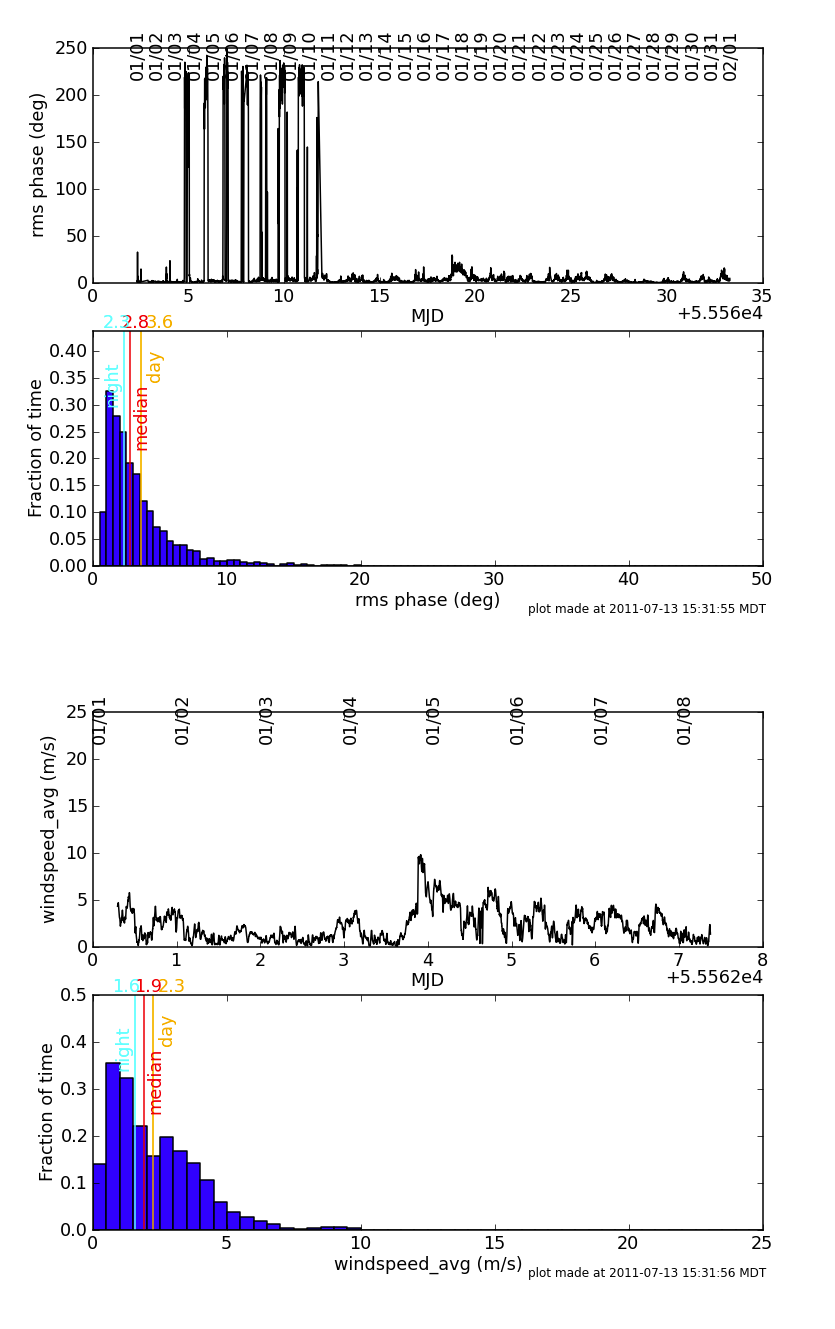
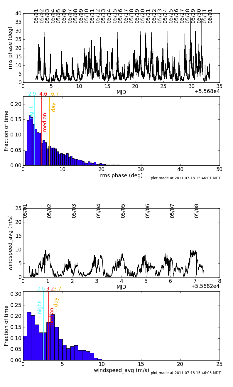
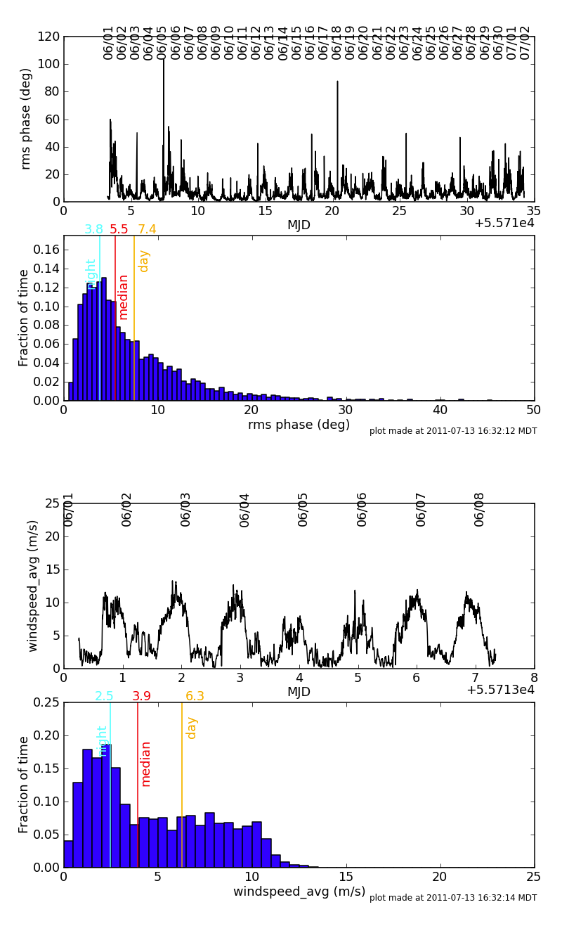
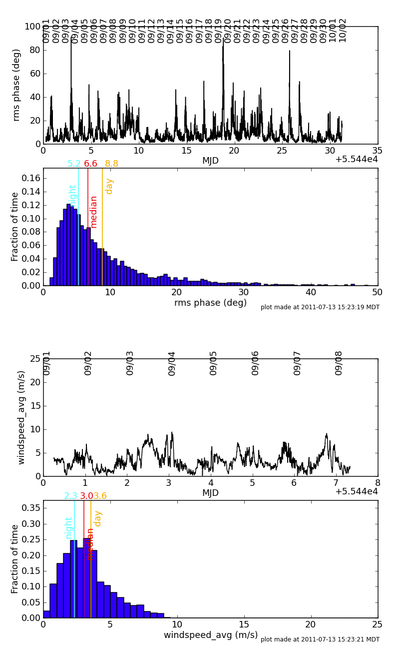
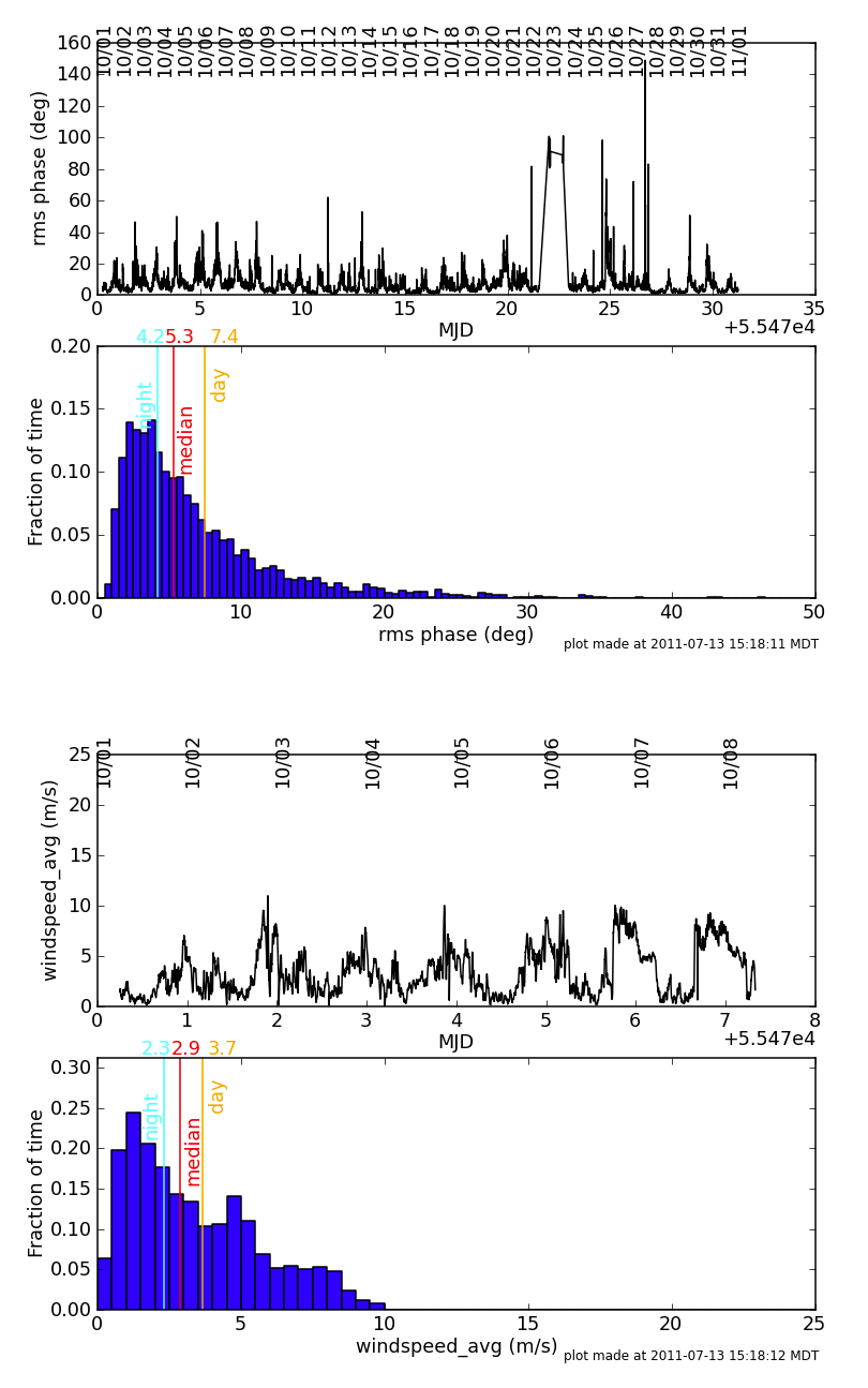
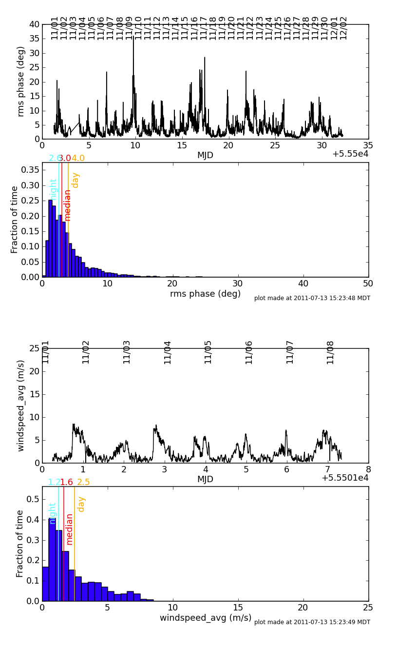
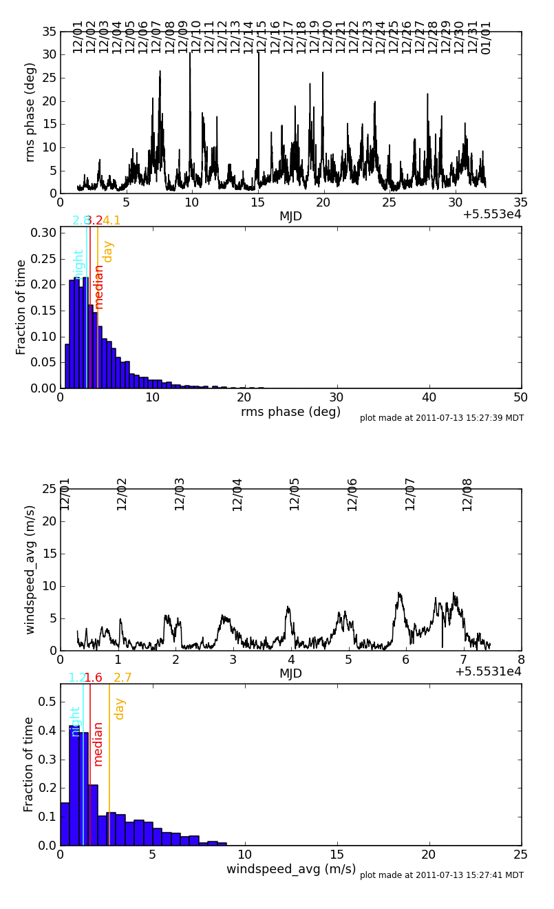
An Atmospheric Phase Interferometer (API) is used to continuously measure the tropospheric contribution to the interferometric phase using an interferometer comprising two 1.5 meter antennas separated by 300 meters, observing an 11.7 GHz beacon from a geostationary satellite. The API data can be used to estimate the required calibration cycle times when using fast switching phase calibration, and in the worst case, to indicate to the observer that high frequency observing may not be possible with current weather conditions. A detailed description of the API may be found at http://www.vla.nrao.edu/astro/guides/api/.
Plots of current/historical data can be found at: https://webtest.aoc.nrao.edu/cgi-bin/thunter/api.cgi
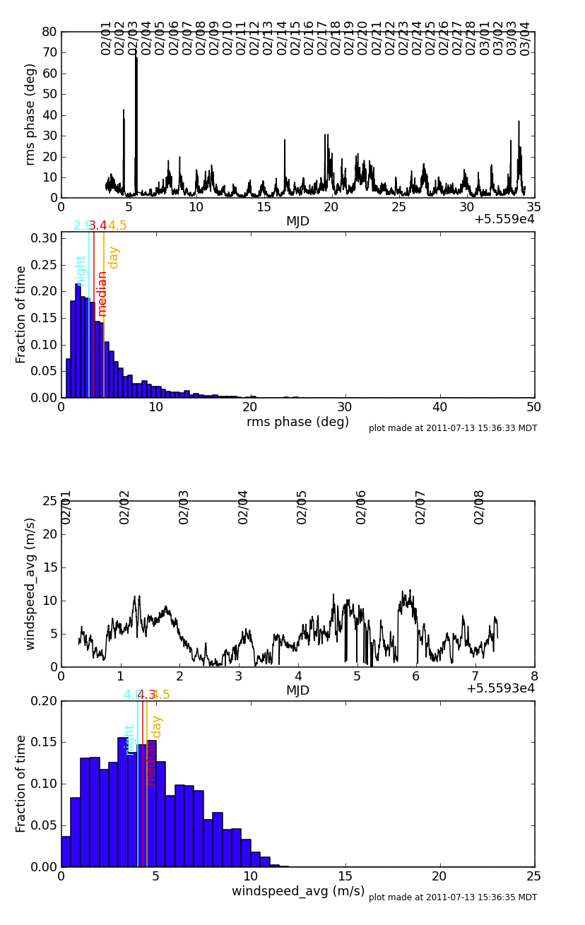
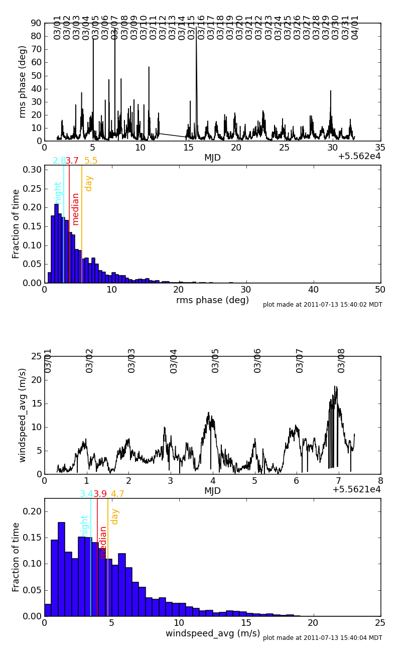
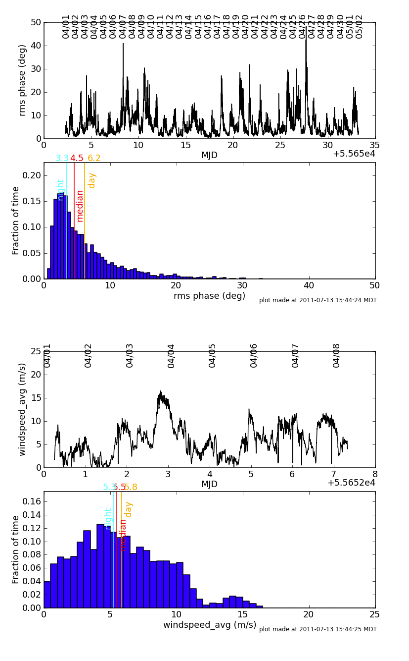
Characteristic seasonal averages are represented below:
| Month | API (night) [deg] | API (median) [deg] | API (day) [deg] | Wind (night) [m/s] | Wind (median) [m/s] | Wind (day) [m/s] |
|---|---|---|---|---|---|---|
| January | 2.3 | 2.8 | 3.6 | 1.6 | 1.9 | 2.3 |
| February | 2.9 | 3.4 | 4.5 | 4.0 | 4.3 | 4.5 |
| March | 2.8 | 3.7 | 5.5 | 3.4 | 3.9 | 4.7 |
| April | 3.3 | 4.5 | 6.2 | 5.3 | 5.5 | 5.8 |
| May | 2.9 | 4.6 | 6.7 | 2.6 | 3.2 | 3.7 |
| June | 3.8 | 5.5 | 7.4 | 2.5 | 3.9 | 6.3 |
| July | 6.2 | 8.3 | 10.5 | 2.9 | 2.9 | 3.0 |
| August | 5.4 | 7.1 | 11.3 | 1.7 | 2.3 | 3.0 |
| September | 5.2 | 6.6 | 8.8 | 2.3 | 3.0 | 3.6 |
| October | 4.2 | 5.3 | 7.4 | 2.3 | 2.9 | 3.7 |
| November | 2.6 | 3.0 | 4.0 | 1.2 | 2.5 | 1.6 |
| December | 2.8 | 3.2 | 4.1 | 1.2 | 1.6 | 2.7 |
Click on the Month links above to see plots of phase and wind speed versus time.
- Note: day indicates sunrise to sunset values; night indicates sunset to sunrise values.
13. Polarization
For projects requiring imaging in Stokes Q and U, the instrumental polarization should be determined through observations of a bright calibrator source spread over a range in parallactic angle. The phase calibrator chosen for the observations can also double as a polarization calibrator provided it is at a declination where it moves through enough parallactic angle during the observation (roughly Dec 15deg to 50deg for a few hour track). The minimum condition that will enable accurate polarization calibration from a polarized source (in particular with unknown polarization) is three observations of a bright source spanning at least 60 degrees in parallactic angle (if possible schedule four scans in case one is lost). If a bright unpolarized unresolved source is available (and known to have very low polarization) then a single scan will suffice to determine the leakage terms. The accuracy of polarization calibration is generally better than 0.5% for objects small compared to the antenna beam size. At least one observation of 3C286 or 3C138 is required to fix the absolute position angle of polarized emission. 3C48 also can be used to fix the position angle at wavelengths of 6 cm or shorter. The results of a careful monitoring program of these and other polarization calibrators can be found at http://www.aoc.nrao.edu/~smyers/evlapolcal/polcal_master.html
High sensitivity linear polarization imaging may be limited by time dependent instrumental polarization, which can add low levels of spurious polarization near features seen in total intensity and can scatter flux throughout the polarization image, potentially limiting the dynamic range. Preliminary investigation of the EVLA's new polarizers indicates that these are extremely stable over the duration of any single observation, strongly suggesting that high quality polarimetry over the full bandwidth will be possible.
The accuracy of wide field linear polarization imaging will be limited, likely at the level of a few percent at the antenna half-power width, by angular variations in the antenna polarization response. Algorithms to enable removable of this angle-dependent polarization are being tested, and observations to determine the antenna polarizations have begun. Circular polarization measurements will be limited by the beam squint, due to the offset secondary focus feeds, which separates the RCP and LCP beams by a few percent of the FWHM. The same algorithms noted above to correct for antenna-induced linear polarization can be applied to correct for the circular beam squint. Measurement of the beam squints, and testing of the algorithms, is ongoing.
Ionospheric Faraday rotation of the astronomical signal is always notable at 20 cm. The typical daily maximum rotation measure under quiet solar conditions is 1 or 2 radians/m2, so the ionospherically-induced rotation of the plane of polarization at these bands is not excessive - 5 degrees at 20 cm. However, under active conditions, this rotation can be many times larger, sufficiently large that polarimetry is impossible at 20 cm with corrrection for this effect. The AIPS program TECOR has been shown to be quite effective in removing large-scale ionospherically induced Faraday Rotation. It uses currently-available data in IONEX format. Please consult the TECOR help file for detailed information. In addition, the interim EVLA receivers generally have poor polarization performance outside the frequency range previously covered by the VLA (e.g., outside the 4.5-5.0 GHz frequency range for C band, and outside 1.3-1.7 GHz for L-band), and the wider frequency bands of these interim receivers may be useful only for total intensity measurements.
For more details see: https://science.nrao.edu/facilities/evla/early-science/polarimetry
14. Correlator Configurations
The EVLA correlator is very flexible, and will be able to provide data in many ways. For the Open Shared Risk Observing (OSRO) program available to the community during the period Sep 2011 through Jan 2013 are offering two independently tunable basebands, where each baseband has up to eight sub-bands. Possible sub-band widths are 128 MHz, 64 MHz, 32 MHz, all the way down in factors of 2 to 0.03125 MHz. All sub-bands must have the same bandwidth and channelization in both basebands, and be contiguous in frequency within each baseband. We will offer three different OSRO modes: full polarization, dual polarization, and single polarization, with 64, 128, and 256 channels per sub-band, respectively. There is always the possibility during offline processing to smooth in frequency to reduce dataset sizes or to improve spectral response.
Starting with the D-configuration in September 2011, we have been providing options for configuring WIDAR for OSRO in the following three ways:
- 1. "OSRO Full Polarization": Four polarization products. This configuration offers 4 polarization products for each sub-band, each of which has 128 MHz bandwidth with 64 channels. It is possible to decrease the subband bandwidth by powers of two, keeping the same number of channels, to provide the capabilities in the following table:
| Sub-band BW (MHz) | Number of channels/poln. product | Channel width (kHz) | Channel width (km/s at 1 GHz) | Total velocity coverage per sub-band (km/s at 1 GHz) |
|---|---|---|---|---|
| 128 | 64 | 2000 | 600/ν (GHz) | 38,400/ν (GHz) |
| 64 | 64 | 1000 | 300 | 19,200 |
| 32 | 64 | 500 | 150 | 9,600 |
| 16 | 64 | 250 | 75 | 4,800 |
| 8 | 64 | 125 | 37.5 | 2,400 |
| 4 | 64 | 62.5 | 19 | 1,200 |
| 2 | 64 | 31.25 | 9.4 | 600 |
| 1 | 64 | 15.625 | 4.7 | 300 |
| 0.5 | 64 | 7.813 | 2.3 | 150 |
| 0.25 | 64 | 3.906 | 1.2 | 75 |
| 0.125 | 64 | 1.953 | 0.59 | 37.5 |
| 0.0625 | 64 | 0.977 | 0.29 | 18.75 |
| 0.03125 | 64 | 0.488 | 0.15 | 9.375 |
- 2. "OSRO Dual Polarization": Two polarization products. This configuration offers 2 polarization products for each sub-band, each of which has 128 MHz bandwidth with 128 channels. It is possible to decrease the sub-band bandwidth by powers of two, keeping the same number of channels, to provide the capabilities in the following table.
| Sub-band BW (MHz) | Number of channels/poln. product | Channel width (kHz) | Channel width (km/s at 1 GHz) | Total velocity coverage per sub-band (km/s at 1 GHz) |
|---|---|---|---|---|
| 128 | 128 | 1000 | 300/ν (GHz) | 38,400/ν (GHz) |
| 64 | 128 | 500 | 150 | 19,200 |
| 32 | 128 | 250 | 75 | 9,600 |
| 16 | 128 | 125 | 37.5 | 4,800 |
| 8 | 128 | 62.5 | 19 | 2,400 |
| 4 | 128 | 31.25 | 9.4 | 1,200 |
| 2 | 128 | 15.625 | 4.7 | 600 |
| 1 | 128 | 7.813 | 2.3 | 300 |
| 0.5 | 128 | 3.906 | 1.2 | 150 |
| 0.25 | 128 | 1.953 | 0.59 | 75 |
| 0.125 | 128 | 0.977 | 0.29 | 37.5 |
| 0.0625 | 128 | 0.488 | 0.15 | 18.75 |
| 0.03125 | 128 | 0.244 | 0.073 | 9.375 |
- 3: "OSRO Single Polarization": One polarization product (new for OSRO observing). It offers 1 polarization product for each sub-band, each of which has 128 MHz bandwidth with 256 channels. It is possible to decrease the sub-band bandwidth by powers of two, keeping the same number of channels, to provide the capabilities in the following table.
| Sub-band BW (MHz) | Number of channels/poln. product | Channel width (kHz) | Channel width (km/s at 1 GHz) | Total velocity coverage per sub-band (km/s at 1 GHz) |
|---|---|---|---|---|
| 128 | 256 | 500 | 150/ν (GHz) | 38,400/ν (GHz) |
| 64 | 256 | 250 | 75 | 19,200 |
| 32 | 256 | 125 | 37.5 | 9,600 |
| 16 | 256 | 62.5 | 19 | 4,800 |
| 8 | 256 | 31.25 | 9.4 | 2,400 |
| 4 | 256 | 15.625 | 4.7 | 1,200 |
| 2 | 256 | 7.813 | 2.3 | 600 |
| 1 | 256 | 3.906 | 1.2 | 300 |
| 0.5 | 256 | 1.953 | 0.59 | 150 |
| 0.25 | 256 | 0.977 | 0.29 | 75 |
| 0.125 | 256 | 0.488 | 0.15 | 37.5 |
| 0.0625 | 256 | 0.244 | 0.073 | 18.75 |
| 0.03125 | 256 | 0.122 | 0.037 | 9.375 |
These capabilities are being provided with integration times no shorter than 1 second in A configuration (3 seconds in B/C/D configurations), and Doppler setting will be available with these correlator configurations.
If it is likely that the data will need to be resampled spectrally in order to Doppler track to a line rest frequency, care should be taken to make sure the spectrum is oversampled to avoid the subsequent introduction of Gibbs ringing or the need to reduce the spectral resolution by Hanning smoothing.
All observations with the EVLA correlator should be treated as traditional VLA spectral line observations, in that they will require observation of a bandpass calibrator. They may also require observation of a delay calibrator. Users should contact NRAO staff for advice on setting up observations with the EVLA correlator.
15. VLBI Observations
VLBI observations with the EVLA, such as phased array and single-antenna (e.g., Y1) modes, have not yet been commissioned and are not yet available to the OSRO program.
16. Snapshots
The two-dimensional geometry of the EVLA allows a snapshot mode whereby short observations can be used to image relatively bright unconfused sources. This mode is ideal for survey work where the sensitivity requirements are modest.
Single snapshots with good phase stability of strong sources should give dynamic ranges of a few hundred. Note that because the snapshot synthesized beam contains high sidelobes, the effects of background confusing sources are much worse than for full syntheses, especially at 20 cm in the D configuration, for which a single snapshot will give a limiting noise of about 0.2 mJy. This level can be reduced by taking multiple snapshots separated by at least one hour. Use of the AIPS program IMAGR or CASA task clean is necessary to remove the effects of background sources. Before considering snapshot observations at 20 cm, users should first determine if the goals desired can be achieved with the existing "Faint Images of the Radio Sky at Twenty-centimeters survey(FIRST, http://www.cv.nrao.edu/first/)" or the "Co-Ordinated Radio 'N' Infrared Survey for High-mass star formation (CORNISH, http://www.ast.leeds.ac.uk/Cornish/public/index.php)" (B configuration), or the NRA VLA Sky Survey (NVSS, http://www.cv.nrao.edu/nvss/) (D configuration, all-sky) surveys.
17. Shadowing and Cross-Talk
Observations at low elevation in the C and D configurations will commonly be affected by shadowing. It is strongly recommended that all data from a shadowed antenna be discarded. This will automatically be done during filling (CASA task importasdm) when using the default inputs (Note: For archival VLA data, the AIPS task FILLM can also flag based on shadowing). AIPS task UVFLG can be used to flag data based on shadowing as well, although it will only flag based on antennas in the dataset, and is ignorant of antennas in other sub-arrays.
Cross-talk is an effect in which signals from one antenna are picked up by an adjacent antenna, causing an erroneous correlation. At 20 cm, this effect is important principally in the D configuration. Careful editing is necessary to identify and remove this form of interference.
18. Combining Configurations and Mosaicing
Any single EVLA configuration will allow accurate imaging up to a scale approximately 30 times the synthesized beam. Objects larger than this will require multiple configuration observations. It is advisable that the frequencies used be the same for all configurations to be combined. Objects larger than the primary antenna pattern may be mapped through the technique of interferometric mosaicing. Time-variable structures (such as the nuclei of radio galaxies and quasars) cause special, but manageable, problems. See the article by Mark Holdaway in reference 2 (Documentation) for more information.
19. Pulsar Observing
Observation of pulsars requiring modes other than those described in Correlator Configurations will not initially be supported on the EVLA.

