test collection

1. Introduction
2. Offered VLA Capabilities during the Next Semester
3. Performance of the VLA during the Next Semester
4. WIDAR Correlator
5. Documentation
6. Contact Information
7. Editor's Notes

Purpose of Document, Older Versions of the OSS

Resolution

The VLA's resolution is generally diffraction-limited, and thus is set by the array configuration and the observing frequency. Like all synthesis arrays, the VLA is sensitive only to structures on a range of angular scales between the diffraction limit (the smallest angular scale detectable) and a "Largest Angular Scale" (which depends on the fringe spacing formed by the shortest baselines in the configuration). For emission structures smaller than the diffraction limit (θ ∼ λ/B_max), the VLA acts like a single-dish instrument—the resulting image is smoothed to the resolution of the array. For emission structures larger than the detectable range, the VLA is simply blind to the emission; this is a limitation unique to interferometers. No subsequent processing can fully recover the missing information from these large scales. It can only be obtained by observing in a more compact VLA array configuration or with data from an instrument that is sensitive to the missing angular scales, such as a large single dish or a compact array of smaller antennas.

Table 3.1.1 displays the VLA's resolution and the scale at which severe attenuation of large-scale structure occurs. This table shows the maximum and minimum antenna separations, the approximate synthesized beam size (full width at half-power; the resolution element) for the central frequency for each band, and the largest angular scale of detectable emission.

These estimates of the synthesized beamwidth are for a uniformly weighted, untapered map produced from a full 12 hour synthesis observation of a source which passes near the zenith.

Notes:

1. B_max is the maximum antenna separation, B_min is the minimum antenna separation, θ_HPBW is the synthesized beam width (FWHM), and θ_LAS is the largest angular scale structure visible to the array.

2. The listed resolutions are appropriate for sources with declinations between −15 and +75 degrees.

3. The approximate resolution for a naturally weighted map is about 1.5 times the numbers listed for θ_HPBW. The values for snapshots are about 1.3 times the listed values.

4. The largest angular scale structure is that which can be imaged reasonably well in full synthesis observations. For single snapshot observations, the quoted numbers should be divided by two.

5. For the C configuration, an antenna from the middle of the north arm is moved to the central pad N1. This results in improved imaging for extended objects, but may slightly degrade snapshot performance. Note that although the minimum spacing is the same as in D configuration, the surface brightness sensitivity and image fidelity to extended structure is considerably inferior to that of the D configuration.

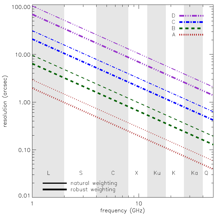
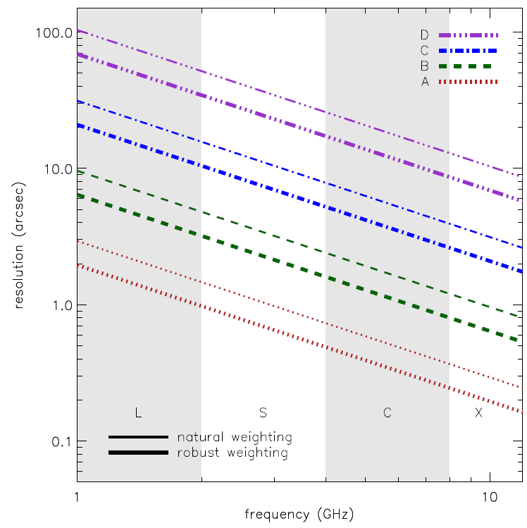
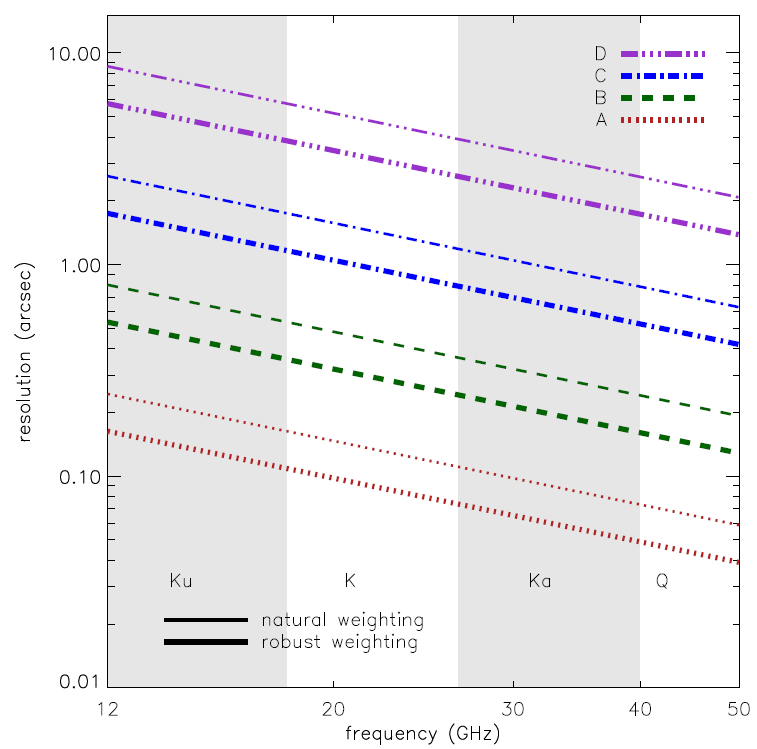
The following figure is a graphical representation of the synthesized beamwidths for natural and robust weighting for the four main array configurations between 1 and 50 GHz. Also available are synthesized beamwidth figures for the low frequency (1–12 GHz) and the high frequency (12–50 GHz) receiver bands.

(click image to enlarge)

Sensitivity

The theoretical thermal noise expected for an image using natural weighting of the visibility data is given by:

where:

- SEFD is the system equivalent flux density (Jy), defined as the flux density of a radio source that doubles the system temperature. Lower values of the SEFD indicate more sensitive performance. For the VLA's 25–meter paraboloids, the SEFD is given by the equation SEFD = 5.62T_sys/η_A, where T_sys is the total system temperature (receiver plus antenna plus sky), and η_A is the antenna aperture efficiency in the given band.

- η_c is the correlator efficiency (~0.93 with the use of the 8-bit samplers).

- n_pol is the number of polarization products included in the image; n_pol = 2 for images in Stokes I, Q, U, or V, and n_pol = 1 for images in RCP or LCP.

- N is the number of antennas.

- t_int is the total on-source integration time in seconds.

- Δν is the bandwidth in Hz.

Figure 3.2.1 shows the SEFDs as a function of frequency used in the VLA exposure calculator for those Cassegrain bands currently installed on VLA antennas, and include the contribution to Tsys from atmospheric emission at the zenith. Figure 3.2.2 shows the SEFDs as a function of frequency for the P-band; these measurements are based on imaging of a field far from the galactic plane. Table 3.2.1 gives the SEFD at some fiducial VLA frequencies.

 Figure 3.2.1: SEFD used in the Exposure Calculator for the VLA. Left: The system equivalent flux density as a function of frequency for the L, S, C and X-band receivers. Right: The system equivalent flux density as a function of frequency for the Ku, K, Ka, and Q-band receivers. SEFDs at Ku, K, Ka, and Q bands include contributions from Earth's atmosphere and were determined under good conditions. 

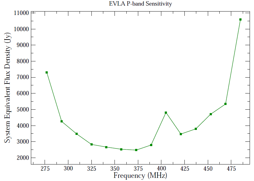
Figure 3.2.2: The SEFD used in the VLA Exposure Calculator as a function of frequency for the P-band receiver

Note that the theoretical rms noise calculated using equation 1 is the best limit possible. There are several factors that will tend to increase the noise compared with theoretical:

• For the more commonly used robust weighting scheme, intermediate between pure natural and pure uniform weightings (available in the AIPS task IMAGR and CASA task clean), typical parameters will result in the sensitivity being a factor of about 1.2 worse than the listed values.
• Confusion. There are two types of confusion: (i) that due to confusing sources within the synthesized beam, which affects low resolution observations the most. Table 3.2.1 shows the confusion noise in D configuration assuming robust weighting (see Condon et al. 2012, ApJ, 758),  which should be added in quadrature to the thermal noise in estimating expected sensitivities. The confusion limits in C configuration are approximately a factor of 10 less than those in Table 3.2.1; (ii) confusion from the sidelobes of uncleaned sources lying outside the image, often from sources in the sidelobes of the primary beam. This confusion primarily affects low frequency observations.
• Weather. The sky and ground temperature contributions to the total system temperature increase with decreasing elevation. This effect is very strong at high frequencies, but is relatively unimportant at the other bands. The extra noise comes directly from atmospheric emission: primarily from water vapor at K-band, and from water vapor and the broad wings of the strong 60 GHz O₂ transitions at Q-band.
• Losses from the 3-bit samplers. The VLA's 3-bit samplers incur an additional 10–15% loss in sensitivity above that expected—i.e., the efficiency factor η_c = 0.78 to 0.83.

In general, the zenith atmospheric opacity to microwave radiation is very low: typically less than 0.01 at L, C, and X-bands; 0.05 to 0.2 at K-band; and 0.05 to 0.1 at the lower half of Q-band, rising to 0.3 by 49 GHz. The opacity at K-band displays strong variations with time of day and season, primarily due to the 22 GHz water vapor line. Observing conditions are best at night and in the winter. Q-band opacity, dominated by atmospheric O₂, is considerably less variable.

Observers should remember that clouds, especially clouds with large water droplets (thunderstorms), can add appreciable noise to the system temperature. Significant increases in system temperature can, in the worst conditions, be seen at frequencies as low as 5 GHz.

Tipping scans—which are currently unavailable but will be implemented at some time in the future—can be used for deriving the zenith opacity during an observation. In general, tipping scans should only be needed if the calibrator used to set the flux density scale is observed at a significantly different elevation than the range of elevations over which the complex gain calibrator (amplitude and phase) and target source are observed.

When the flux density calibrator observations are within the elevation range spanned by the science observing, elevation dependent effects (including both atmospheric opacity and antenna gain dependencies) can be accounted for by fitting an elevation-dependent gain term. See the following items:

• Antenna elevation-dependent gains. The antenna figure degrades at low elevations, leading to diminished forward gain at the shorter wavelengths. The gain-elevation effect is negligible at frequencies below 8 GHz. The antenna gains can be determined by direct measurement of the relative system gain using the AIPS task ELINT on data from a strong calibrator which has been observed over a wide range of elevation. If this is not possible, care should be taken to observe a primary flux calibrator at the same elevation as the target.

  Both CASA and AIPS allow the application of elevation-dependent gains and an estimated opacity generated from ground-based weather through the CASA tasks gencal and plotweather, and AIPS task INDXR.

• Pointing. The SEFD quoted above assumes good pointing. Under calm, nighttime conditions, the antenna blind pointing is about 10 arcsec rms. The pointing accuracy in daytime can be much worse—occasionally exceeding 1 arcminte due to the effects of solar heating of the antenna structures. Moderate winds have a very strong effect on both pointing and antenna figure. The maximum wind speed recommended for high frequency observing is 11 mph (5 m/s). Wind speeds near the stow limit 45 mph (20 m/s) will have a similar negative effect at 8 and 15 GHz.

To achieve increased pointing accuracy, referenced pointing is recommended where a nearby calibrator is observed in interferometric pointing mode every hour or so. The local pointing corrections measured can then be applied to subsequent target observations. This reduces rms pointing errors to as little as 2–3 arcseconds (but more typically 5–7 arcseconds) if the reference source is within about 15 degrees in azimuth and elevation of the target source and the source elevation is less than 70 degrees. At source elevations greater than 80 degrees (zenith angle < 10 degrees), source tracking becomes difficult; it is recommended to avoid such source elevations during the observation preparation setup.

Use of referenced pointing is highly recommended for all Ku, K, Ka, and Q-band observations, and for lower frequency observations of objects whose total extent is a significant fraction of the antenna primary beam. It is usually recommended that the referenced pointing measurement be made at 8 GHz (X-band), regardless of what band your target observing is at, since X-band is the most sensitive and the closest calibrator is likely to be weak. Proximity of the reference calibrator to the target source is of paramount importance; ideally the pointing sources should precede the target by 20 or 30 minutes in Right Ascension (RA). The calibrator should have at least 0.3 Jy flux density at X-band and be unresolved on all baselines to ensure an accurate solution.

To aid VLA proposers there is an online guide to the exposure calculator; the exposure calculator provides a graphical user interface to these equations.

Special caveats apply for P-band (230–470 MHz) observing. The SEFD's in Figure 3.2.2 or that listed in table 3.1.2 are from an observation taken far from the Galactic plane, where the sky brightness is about 30K. At P-band, Galactic synchrotron emission is very bright in directions near the Galactic plane. The system temperature increase due to Galactic emission will degrade sensitivity by factors of two to three for observations in the plane, and by a factor of five or more at or near the Galactic center. Additionally, the antenna efficiency (currently about 0.31 for 300 MHz) will decline with both increasing and decreasing frequencies from the center of P-band.

The beam-averaged brightness temperature measured by a given array depends on the synthesized beam, and is related to the flux density per beam by:

where T_b is the brightness temperature (Kelvins) and Ω is the beam solid angle. For natural weighting (where the angular size of the approximately Gaussian beam is ∼1.5λ/B_max), and S in mJy per beam, the parameter F depends on the synthesized beam, therefore on the array configuration, and has the approximate value of F = 190, 18, 1.7, 0.16 for A, B, C, and D configurations, respectively. The brightness temperature sensitivity can be obtained by substituting the rms noise, ΔI_m, for S. Note that Equation 2 is a beam-averaged surface brightness; if a source size can be measured, then the source size and integrated flux density should be used in Equation 2 and the appropriate value of F calculated. In general, the surface brightness sensitivity is also a function of the source structure and how much emission may be filtered out due to the sampling of the interferometer. A more detailed description of the relation between flux density and surface brightness is given in Chapter 6 of Reference 1, listed in Documentation.

For observers interested in HI in galaxies, a number of interest is the sensitivity of the observation to the HI mass. This is given by van Gorkom et al. (1986; AJ, 91, 791):

where D is the distance to the galaxy in Mpc, and SΔV is the HI line area in units of Jy km/s.

Bands

For observations taken with the 8-bit samplers, each receiver can tune to two different frequencies, each 1024 MHz wide, within the same frequency band. Right-hand circular (RCP) and left-hand circular (LCP) polarizations are received for both frequencies, except for the low-band receiver (50–500 MHz), which provides linear polarization (X and Y). Each of these four data streams follows the VLA nomenclature and are known as IF (for Intermediate Frequency channel) A, B, C, and D. IFs A and B provide RCP (or Y when applicable), IFs C and D provide LCP (or X when applicable). IFs A and C are always at the same frequency, as are IFs B and D (but note that the A and C IFs frequency is usually different from the B and D frequency). We normally refer to these two independent data streams as IF pairs, i.e., the A/C pair and the B/D pair. In 8-bit mode, a maximum of 1024 MHz can be correlated for each IF pair (see the WIDAR Section), for a total maximum bandwidth of 2048 MHz. To distinguish this 8-bit system from the 3-bit system, these IF pairs are denoted A0/C0 and B0/D0.

More options are available with the 3-bit samplers. This system provides four (R,L) polarization pairs, each 2048 MHz wide. The A/C IF pair provides two sampled pairs, labelled A1/C1 and A2/C2, and the B/D IF pair provides two sampled pairs, labelled B1/D1 and B2/D2.

For more details on the 8-bit and 3-bit samplers see the VLA Samplers section.

The tuning ranges, along with default frequencies for continuum applications, are given in Table 3.3.1 below.

Table 3.3.1: Default frequencies for continuum applications

Band	Range1	8-bit continuum applications (GHz)		3-bit continuum applications (GHz)
	(GHz)	IF pair A0/C0	IF pair B0/D0	IF pair A1/C1	IF pair A2/C2	IF pair B1/D1	IF pair B2/D2
4 m (4)	0.054 – 0.0842	—	.070 – .082	—	—	—	—
90 cm (P)	0.20 – 0.503	0.224 – 0.4803	—	—	—	—	—
4 m (4)/90 cm (P)	0.054 – 0.0842/ 0.20 – 0.503	0.224 – 0.4803	.070 – .082
20 cm (L)	1.0 – 2.04	1.0 – 1.54	1.5 – 2.04	—	—	—	—
13 cm (S)	2.0 – 4.0	2.0 – 3.0	3.0 – 4.0	—	—	—	—
6 cm (C)	4.0 – 8.0	4.5 – 5.5	5.5 – 6.5	4.0 – 6.0	6.0 – 8.0	—	—
3 cm (X)	8.0 – 12.0	8.0 – 9.0	9.0 – 10.0	8.0 – 10.0	10.0 – 12.0	—	—
2 cm (Ku)	12.0 – 18.0	13.0 – 14.0	14.0 – 15.0	12.0 – 14.0	14.0 – 16.0	—	16.0 – 18.0
1.3 cm (K)	18.0 – 26.5	20.2 – 21.2	21.2 – 22.2	22.0 – 24.0	24.0 – 26.0	18.0 – 20.0	20.0 – 22.0
1 cm (Ka)	26.5 – 40.0	32.0 – 33.0	31.0 – 32.0	33.0 – 35.0	35.0 – 37.0	29.0 – 31.0	31.0 – 33.0
0.7 cm (Q)	40.0 – 50.0	40.0 – 41.0	41.0 – 42.0	44.0 – 46.0	46.0 – 48.0	40.0 – 42.0	42.0 – 44.0

Notes:

1.  Listed here are the nominal band edges. For all bands, the receivers can be tuned to frequencies outside this range, but at the cost of diminished performance. Contact the NRAO Helpdesk for further information.

2. The 4-band system is currently under development. The default frequency range maximizes sensitivity of the system and provides a nominal bandwidth of 12 MHz and a channel resolution of 64 kHz.

3. The default setup for P-band will provide 16 subbands from the A0/C0 IF pair, each 16 MHz wide, to cover the frequency range 224–480 MHz. The channel resolution is 125 kHz. 

4. The default frequency setup for L-band comprises two 512 MHz IF pairs (each comprising 8 contiguous subbands of 64 MHz) to cover the entire 1–2 GHz of the L-band receiver.

Tuning Restrictions

In general, for all frequency bands except Ka, if the total span of the two independent IF pairs of the 8-bit system (defined as the frequency difference between the lower edge of one IF pair and the upper edge of the other) is less than 8.0 GHz, there are no restrictions on the frequency placements of the two IF pairs. For K, Ka, and Q-bands—the only bands where a span greater than 8 GHz is possible—there are special rules:

• At Ka-band, the low frequency edge of the A0/C0 IF pair must be greater than 32.0 GHz. There is no restriction on the B0/D0 frequency, unless the B0/D0 band overlaps the A0/C0 band when the latter is tuned at or near the 32.0 GHz limit. In this case, the Observation Preparation Tool (OPT) may not allow the requested frequency setups. Users wanting to use such a frequency setup are encouraged to contact the NRAO Helpdesk for possible tuning options.
• At K and Q-bands, if the frequency span is greater than 8.0 GHz, the B0/D0 frequency must be lower than the A0/C0 frequency.

For the 3-bit system, the maximum frequency span permitted for the A1/C1 and A2/C2 IF pairs is about 5000 MHz. The same restriction applies to B1/D1 and B2/D2. The tuning restrictions given above for the separation and location of the 8-bit pairs A0/C0 and B0/D0 also apply to the 3-bit pairs, with A0/C0 replaced by A1/C1 and A2/C2, and B0/D0 replaced by B1/D1 and B2/D2.