
Dynamic Scheduling Considerations
1. Introduction to Dynamic Scheduling
Most scheduling blocks (SBs) are observed dynamically, based on factors that NRAO controls and on factors that the observer controls. Such dynamic scheduling enhances science data quality and the array's ability to discharge time-sensitive science. On rare occasions, an SB that requires coordinated observations with other telescopes will be scheduled on a fixed sidereal date.
NRAO staff use the Observation Scheduling Tool (OST) to examine the current observing conditions and the queue of SBs submitted for the current array configuration. The observing conditions are quantified by the RMS phase measured with the Atmospheric Phase Interferometer (API), the wind speed, and the sunrise/sunset time. The OST then applies heuristics to create a schedule, which is just a time series of optimal SBs. The first optimal SB in the series is then sent off for execution by the monitor and control system. Just before that execution completes, the OST again applies heuristics to create a new schedule.
The heuristics used by the OST include the scheduling priority (A, B, or C) assigned by the Time Allocation Committee and the linear-rank score assigned by the Science Review Panel. The heuristics also include SB attributes under observer control, specifically its duration, weather constraints (API and wind limits), observing bands, range of LST start times and, optionally, an earliest start date and a request to avoid sunrise/sunset. The observer can also convey comments to the operator, for example to instruct the operator not to execute the SB for some reason if it has been selected from the queue.
Dynamic scheduling obviously means that the observer does not know when the observations will occur. This must be kept in mind when preparing an SB. In particular, the observer should check that none of the possible LST start times create problems with antenna wraps and the scans of the flux density scale calibrator. These topics are discussed in more detail below.
2. Doppler Correction
For some spectral line setups, Doppler correction (position and velocity) should be applied. The benefit of Doppler Setting, since the VLA is dynamically scheduled, is that it calculates the sky frequency at the beginning of an SB and keeps this fixed for the duration of the SB. Doppler Setting can be specified for each individual baseband in the OPT, removing the burden to do this for each possible observing run by the observer. For more details, refer to the Doppler Correction section within the Spectral Line guide.
3. Antenna Shadowing
An antenna is shadowed when its line-of-sight to the source is partially or fully blocked by another antenna in front of it. The shadowed antenna will collect less radiation from the source than if it had not been shadowed, reducing the sensitivity on the baselines to that antenna. Shadowing is more likely to occur when sources are at low elevation and when the antennas are in more compact configurations. The OPT will report, per scan, the maximum amount of shadowing, if any, will occur according to the location in the sky of the target and the configuration of the observations. D-configuration is affected by shadowing more than the other configurations because the antennas are at their closest proximity to each other. If you select "Any" configuration, the OPT will calculate the worst-case scenario by assuming the D-configuration to calculate shadowing.
If any calibration scans will be shadowed for any of the valid LST start times, we recommend increasing the observing time of the calibration source to account for the loss of sensitivity. Table 2.1 shows the amount of shadowing in respect to the fraction of an antenna that is blocked with the corresponding loss of sensitivity. All shadowed baselines will be similarly affected. Note that the loss of sensitivity is not linear with the fractional shadowing.
| Shadowing | Fraction of Area Blocked | Baseline Sensitivity Loss |
|---|---|---|
| 1 m | 0.01 | 0.5% |
| 5 m | 0.10 | 5% |
| 12.5 m | 0.39 | 22% |
| 18 m | 0.64 | 40% |
| 25 m | 1 | 100% |
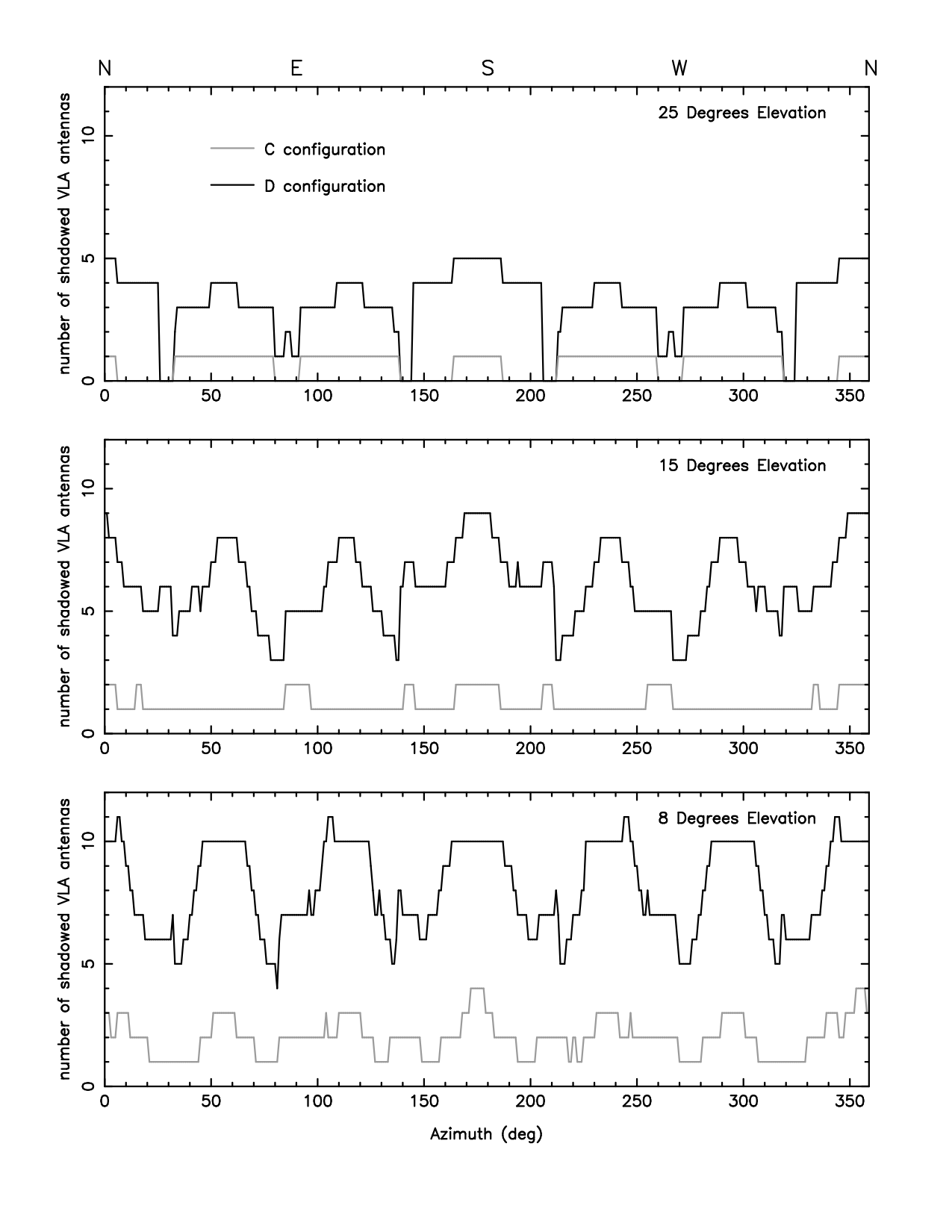
Avoiding antenna shadowing during the D-configuration relies on the azimuth of the antennas, which is dependent on the location of the source and the LST start time. Therefore, to guarantee no more than a single shadowed antenna, restrict the elevations, if possible, to >40° for D-configuration and >25° for C-configuration. Shadowing is worst along the azimuths of the arms (in both directions), so has a six-fold symmetry. See Figure 2.1 below. Note that the maximum elevation (in degrees) for your target is its Declination plus 56°, so it may not be possible to avoid any shadowing for sources at Dec < -16° or Dec < -31° for D and C configuration, respectively.
 |
|
Figure 2.1: Plot of shadowed azimuths in D-configuration (black line) and C-configuration (grey line), for three elevations: 25°, 15°, and 8°. (Important note, these plots and the post processing packages (AIPS and CASA) do not calculate shadowing flags for an antenna placed on the Master Pad or the antenna barn.) |
4. Antenna Wraps
Introduction
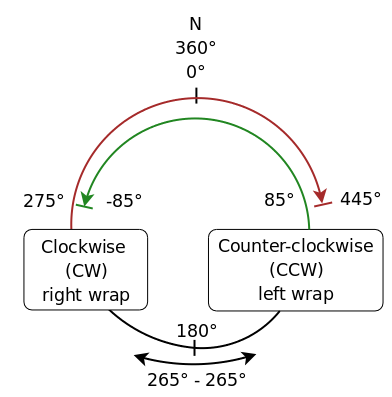
To help avoid confusion, we will define some terminology. For a visualization of these terms, refer to the wrap diagram below (Figure 2.4.1).
| Wrap Type | Definitions |
|---|---|
|
Clockwise (CW) Right or Outer |
When looking down at the VLA from above, the antennas on a CW wrap would appear to be tracking in azimuth in a CW direction from 180° real AZ. |
|
Counter-clockwise (CCW) Left or Inner |
When looking down at the VLA from above, the antennas on a CCW wrap would appear to be tracking in azimuth in a CCW direction from 180° real AZ. |
| North | This term is used where the CW and CCW wraps overlap between 275° and 85° real AZ, passing through 0° / 360° (north) (CW: 275° to 445° (85° real AZ) / CCW: −85° (275° real AZ) to 85°). |
| South | This term is used for the unambiguous section of the wraps where there is no preference over the use of either CW or CCW wraps. The south wrap is from 85° to 275° real AZ, passing through 180° (south). |
During the observation of a single source, or by switching from one source to the next, the antennas are continuously changing their pointing toward different directions in the sky. The cables for power, communication, and data transfer have a limited length and wrap around the rotation (azimuth) axis of the antenna while the antenna moves. Software directs the antenna movements to prevent them from tightening and snapping when the cables reach the azimuth cable wrap limit, i.e., when they have wrapped ±265° either direction (CW or CCW) from the south (at 180° real azimuth). At a wrap limit, instead of continuous tracking during a scan or directly moving to the next scan at a scan boundary, the antennas will move the opposite long way while unwrapping the cables. As the azimuth slew rate is 40°/min, a full 360° azimuth unwrap will take up 9 minutes (plus some settling time) of unusable observing time. It is important to avoid such a situation and pay attention to the antenna azimuth and wrap during the observation, which means paying attention to the wrap when the azimuth of the scan in the Schedule Summary reports if the scans approach 85° and 445°, or when the scan sequence crosses −85° and 275° azimuth (see Figure 2.4.1 below). Perhaps experiment with different azimuth (and elevation) starting positions to investigate the effect (and starting slew times) for a particular scheduling block (SB). Note: if adjustments are made to the starting azimuth and elevation positions of the SB, please return them to the default positions of 225° azimuth and 35° elevation.
Another inconvenient wrapping situation appears when observations near zenith (elevations larger than about 80°) switch between sources on different azimuth wraps. This happens when a target and calibrator are close to, but on opposite sides of 34.1° (34°04′43.497′′) declination (latitude of the VLA). The OPT will show slew times much longer than expected for the angular source separation, and indicate an azimuth wrap (CW or CCW) on only one of the sources in the reports of the scan list. So even if a calibrator may be a bit further away or less strong, it may be the better option when it is on the same side of zenith. Experiment with different LST start times to investigate the effect for a particular SB if no suitable calibrator can be found on the same side of zenith.
The most important antenna wrap issue arises at the start of the SB as the wrap chosen determines the wrap for the rest of the observation (if not specified in further scans). This wrap should also align the azimuth of antennas combined from previous different subarrays at the start of observing. At the end of the previous program the antennas (or subarrays of antennas) are left pointing in a direction that is dependent on the previous program, and may be any azimuth between −85° and +445°. When the antennas slew toward the first source in the SB, there are two options: clockwise (CW, also known as Right or Outer) or counterclockwise (CCW, also known as Left or Inner); see Figure 2.4.1. In dynamic scheduling, the software will choose the shortest slew to the first source unless otherwise specified in the antenna wrap option in the first scan(s) in the SB. This default software choice may or may not be the optimum case for the observations. To avoid problems, if any of the scans in the SB are observed outside the range between +85° and +275° in the south, then specify the antenna wrap at the start-up sequence to be assured that thereafter the wraps in the reports listing correspond to the actual wraps during the observations. Only when all scans in the SB remain between, or completely avoid the range of +85° and +275° azimuth during any of the start times specified in the LST start range, there is no explicit need to specify any wrap. That is, observations entirely on the south wrap or entirely on the north wrap should be fine, but if you include any of the common standard flux density scale calibrators (i.e., 3C48 or 3C286) most likely the observation will include LSTs where these sources are on the other wrap.
Quick Guide
When to request an antenna wrap: Unless the first source (i.e., setup scan(s) and the first standard observing or reference pointing scan) is always in the unambiguous (south) part of the wrap (85° ≥ AZ ≤ 275°; see Figure 2.4.1 below) during any LST start time within the set range, then you should request an antenna wrap for each scan of the start-up sequence (generally the first 10–15 minutes of the SB). If the SB starts with either 3C286 or 3C48, then an antenna wrap should be selected and continue to specify that wrap for the startup sequence of the SB. Be aware that when 3C286 or 3C48 rise and set they cross the ambiguous (275° ≥ AZ ≤ 85°; see Figure 2.4.1 below) part of the wrap, which can cause problems with unwrapping to the next source (i.e., the complex gain calibrator), so there may not be any time on the first complex gain calibrator scan or the first science target scan.
Which antenna wrap to choose: Look at the first scan under the Schedule Summary report to check if there is an unwrap issue (275° ≥ AZ ≤ 85°) for all times in the LST start range. Follow how the azimuth evolves during the observing block and whether it crosses the 275°/85° boundaries. Select a wrap which takes the antennas in a direction so there is plenty of room for the antennas to move without having to unwrap again; check the LST start range by stepping through at least every hour, making sure that all scans have plenty of on source time (no less than 20sec for standard observing and no less than 2min30sec for reference pointing). Sometimes the LST start range will need to be adjusted to avoid an unwrap.
Antenna Wrap Caveats: When the schedule summary reports a calculated wrap CW or calculated wrap CCW, do not assume that the calculated wrap will be the starting wrap. The calculated wrap is also a good indication that a wrap should be set, but not always in the calculated direction. Do not be alarmed if you request a wrap and it does not appear in the schedule summary report.
Addressing Both Wraps: When an SB can have two LST start ranges to cover the rising and setting of sources, we recommend submitting two SBs to cover the two LST start ranges and their corresponding antenna wraps. For more details on how to create linked SBs, refer to the FAQs page or the Linking SBs section of the OPT manual.
Antenna Wrap Bugs in the OPT:
- In some circumstances, and only for the first and second scan, there is a discrepancy in the reporting of the telescope azimuth. This is apparent when an SB starts on a source that is always in the north (dec > 34°) using the default of azimuth 225° (i.e., in the south). In this case, the OPT may report a confusing starting azimuth on the first scan and an azimuth jump and/or a wrap change for the second scan (even if it is the same source). This bug can be ignored and no wrap need be set.
- A slightly different wrap display bug in the Reports page, is where the first and second scan on the north wrap may differ by 360°.
Detailed Guide
Wrap Diagram
Figure 2.4.1 shows the antenna wrap diagram; this diagram is very helpful in resolving wrap issues. Use this diagram in conjunction with the azimuth column in the scan listing of the Schedule Summary Report table for different LST start times to investigate whether any wrap issues may occur. Often wrap issues will appear when the standard flux density scale calibrator sources 3C286 and 3C48 are scheduled to be observed at rise and/or set at either limit of the LST start range, or when they might be observed during culmination at zenith. That is, many observers should take note to avoid any problems by adhering to the antenna wrap guidelines.
It should be noted, for completeness, that the online software monitors the azimuth of the antennas constantly (i.e., on time scales of seconds; not per scan). As soon as the actual azimuth of a particular antenna hits the −85° or +445° azimuth limit, the antenna will be directed to unwrap and slew in the opposite direction to catch up with the observation instruction. As this happens at the actual azimuth (after the global pointing model and possible additional reference pointing corrections are applied), the time at which a specific (the first) antenna might unwrap may be different from another antenna (the last) by a minute or so. To avoid unwrapping antennas at different times, make sure the scans do not start or stop very close to these azimuth limits for any of the potential LST start times of the SB.
|
West |
 |
East |
| Figure 2.4.1: VLA wrap diagram with Azimuth conventions and readings and the cable wrap limits. Clockwise wrap goes over West (red; outermost curve from the bottom to the top of the spiral) and Counterclockwise over East (green; innermost curve). South (unambiguous) wrap is between azimuth +85° and +275° (black; bottom of the spiral) and North (ambiguous) wrap is in the area at the top, between −85° and +85° or +275° and +445°. | ||
Antenna Wrap & Elevation Considerations
A source is rising when the LST (modulus 24h) is less than the RA of the source. A source is setting when the LST is greater than the RA of the source. Note that for this reasoning, the RA and LST (range) should be within 12h of each other to properly determine rise or set. If the difference is larger, add 24h to either the RA or LST range values, whichever has the lower value in the SB.
- If all of your sources, targets, and calibrators have declinations below about 8.5°, they are all observed in the south wrap and will never reach the ambiguous wrap region: no wrap setting is needed. Note that this almost never happens as you want to include one of your flux density scale calibrators and all have a declination larger than 8.5°. If any of the sources has a declination very close to 8–9°, this rule of thumb may not apply and more care should be taken in checking the observing schedule. This 8.5° limit assumes observations all the way down to the elevation limit of 8°. For observations using higher elevation limits, the 8.5° declination rule becomes a higher-than-nine declination rule, depending on the actual elevation limit:
|
|
Elevation limit | 8° | 10° | 15° | 20° | 25° | 35° | 45° | 60° | 90° |
l=latitude (34o04' for VLA) |
|---|---|---|---|---|---|---|---|---|---|---|---|
| Highest Dec. on the south wrap (Az=85°) | +8°35' | +9°41' | +12°24' | +15°02' | +17°35' | +22°21' | +26°34' | +31°25' | +34°04' | sin(d)=sin(l)sin(e)+cos(l)cos(a)cos(e) or for VLA approximately sin(d)=0.5602*sin(e)+0.0722*cos(e) | |
| Lowest observable Dec. (Az=180° south) | -48° | -46° | -41° | -36° | -31° | -21° | -11° | +4° | +34° |
d=e+l-90, or for VLA d=e-55o56' |
|
| Circumpolar Declination (on north wrap) | +64° | +66° | +71° | +78° | +81° | (+90°) | d=e+90-l, or for VLA d=e+55o56' | ||||
- If all of your sources (targets and calibrators) have declinations above about 34°, they are all observed in the north wrap and will never use the south wrap region: no wrap setting is needed. Note that this is unlikely unless you use 3C147 as your flux density scale calibrator or 3C295 (in the case you observe only below 2 GHz in D configuration). If any of the sources has a declination very close to 34°, this rule of thumb may not apply and more care should be taken in checking the observing schedule.
- If your first source has a declination of less than about 34° and is rising at the start of the observation, set the starting sequence wraps (first 10–15 minutes worth of scans at the start of the block) to CCW (left). If the first source is setting, set the wrap to CW (right).
- If your first source has a declination of more than about 34° (i.e., it will be observed in the north), then there are two options that will only make a difference once the next source in the sequence has a declination below about 34° (otherwise you can use the second rule above). If that next southern declination source at the time of the observing LST (i.e., the starting LST time plus the duration of time into the observation) is rising then set the starting sequence (first 10–15 minute worth of scans at the start of the block) wraps to CCW (left). If this southern source is setting, set the beginning sequence wraps to CW (right).
Always make sure to check the wraps in the Reports tab of the SB in the OPT. If in doubt or confused, please leave the wrap designation to "No Preference" and consult the NRAO Helpdesk.
For more detailed information on setting antenna wraps, see the section How to Proceed below.
Wrap Issues & Standard Flux Density Scale Calibrators
The default standard flux density scale calibrators for the VLA, 3C286 (J1331+3030) and 3C48 (J0137+3309), are nicely separated by about 12 hours in Right Ascension (RA) but, unfortunately, have two major inconveniences. First, their declination is almost the latitude of the VLA (34.1°), which causes them to culminate almost at zenith on the southern wrap and, second, while they are mostly in the southern wrap, they rise and set in the northern wrap. Catching these flux density scale calibrators in short SBs may be difficult for target observations in certain regions distant from these calibrators on the sky. Therefore, it quite often happens that the flux density scale calibrator is observed in these dynamic SBs when a flux density scale calibrator just rises or just sets, where wrap issues may become a problem for targets on the southern wrap. For targets on the northern wrap, even though the flux density scale calibrators may be high in the sky, it decreases the usable LST start range to place the flux density scale calibration scans if wrap issues are to be avoided. See Table 2.4.2 and Figure 2.4.2 for details.
Table 2.4.2: Wraps and wrap limits for Standard Flux Density Scale Calibrators at the VLA
| North Wrap | South Wrap | North Wrap | ||||||
|---|---|---|---|---|---|---|---|---|
| RISE AT | AZ= 85/445° | AZ= −85/275° | SET AT | |||||
| AZ | LST | LST | EL | EL | LST | LST | AZ | |
| 3C48 | 55/415° | 18:42 | 23:53 | 68° | 68° | 03:23 | 08:33 | −56/304° |
| 3C286 | 59/419° | 06:45 | 10:53 | 57° | 57° | 16:09 | 20:18 | −58/302° |
| 3C138† |
75/435° | 23:16 | 00:29 | 23° | 23° | 10:13 | 11:27 | −75/285° |
† 3C138 has varied in flux density over the last few years, but appears to have settled back to its original flux density.
| RISE AT | EASTERNMOST AZIMUTH | WESTERNMOST AZIMUTH | SET AT | |||
|---|---|---|---|---|---|---|
| AZ | LST | LST | AZ | |||
| 3C147 | 33/393° | 21:32 | 51/411° | −51/309° | 13:53 | −33/327° |
| 3C295‡ | 30/390° | 05:45 | 48/408° | −48/312° | 22:38 | −30/330° |
‡ 3C295 is only useful at low frequencies and short baselines, i.e., typically at P- and L-band in D configuration.
Note: CASA does not have a flux density scale model for 3C295.
 |
|
Figure 2.4.2: Antenna wrap as function of LST for the standard calibrators. (Click image for a larger view.) |
When the source is observed at an LST shown in green in Figure 2.4.2 (above), the source is in the south and typically no wrap issues arise. When the LST is red, the source is in the northern wrap and either a CCW (left; at rise) or a CW (right; at set) wrap should be specified in the scan. For 3C147 and 3C295 the wrap should be specified as well; the wrap, however, will depend on the efficiency to reach the other sources specified in the schedule. The yellow LST regions are when the sources, 3C48 and 3C286, are at an elevation above 80° and should probably be avoided during high frequency observing. (Note, low frequency observing can observe up to 85° in elevation, too much higher in elevation can cause antenna wrap issues.)
How to Proceed
Initially, it is best not to worry about the antenna wrap until the SB has been created. Then extensively check the azimuth of the scans in the SB for all LST start times in the anticipated LST start time range. This action will reveal if any wrap issues occur for some or all of the possible LST start times.
Aside from any wrapping issues, remember that 3C286 and 3C48 culminate near zenith. To avoid pointing problems at high elevations (≥ 80°) during high frequency observations, it is probably best to avoid having scans for these flux density scale calibrators during the LST range 12:47–14:15 for 3C286 and the range 00:50–02:25 for 3C48. Restrict the LST start range so the scans with 3C286 and/or 3C48 will not happen for these LST times, or perhaps even split the LST start range in two (or more) non-overlapping LST start ranges in the INFORMATION tab of the SB. Ideally, one would want to observe the flux density scale calibrator at about the same elevation as the target sources to obtain a more accurate flux density, especially at the higher frequencies. However, this is hard to plan and not always manageable with dynamic scheduling: it would require a restricted LST start range which would decrease observing chances. Another suggestion, for similar reasons, is to try and observe the flux density or bandpass calibrator when the target source passes through zenith (if its declination is near 34°).
Assuming that the target sources are not scattered all over the sky (e.g., for a survey), there are essentially four cases when using 3C286, 3C48, and/or 3C138:
- 3C286/3C48 can only be observed between rise and culmination in the (South)East: The target source is leading the flux density scale calibrator in the south or north of zenith, typically by up to 6 hours in RA (otherwise the other flux density scale calibrator is more likely to be chosen).
- For dec < 34.1° the target source will be south of zenith and set after the flux density scale calibrator rises. There should be no wrap issues if the wrap directs the antennas to observe the flux density scale calibrator in the CCW (left) wrap or when the LST start range is limited such that the flux density scale calibrator scan can only happen after the LST time for AZ = 85°/445° for that flux calibrator in the table above. Typically, the flux density scale calibrator is observed at the end of the SB.
- For dec > 34.1° the target source will be north of zenith and stay on the north wrap. There should be no wrap issues if the flux density scale calibrator is observed before the LST time for AZ = 85°/445° for that flux density scale calibrator in the table above. Typically the flux density scale calibrator is observed whenever the scan can fit in the LST range for the eastern north wrap, i.e., between rise time LST and the LST time for AZ = 85°/445° for that flux density scale calibrator in the table above.
- 3C286/3C48 can only be observed between culmination in the (South)West and set: The target source is trailing the flux density scale calibrator in the south or north of zenith, typically by up to 6 hours in RA (otherwise the other flux density scale calibrator is more likely to be chosen).
- For dec < 34.1° the target source will be south of zenith and rise before the flux density scale calibrator sets. There should be no wrap issues if the wrap directs the antennas to observe the flux density scale calibrator in the clockwise CW (right) wrap or when the LST start range is limited such that the flux density scale calibrator scan can only happen before the LST time for AZ = −85°/275° for that flux density scale calibrator in the table above. Typically, the flux density scale calibrator is observed at the start of the SB.
- For dec > 34.1° the target source will be north of zenith and stay on the north wrap. There should be no wrap issues if the flux density scale calibrator is observed after the LST time for AZ = −85°/275° for that flux density scale calibrator in the table above. Typically the flux density scale calibrator is observed whenever the scan can fit in the LST range for the western north wrap, i.e., between the LST time for AZ = −85°/275° and set time LST for that flux density scale calibrator in the table above.
- 3C286/3C48 can be observed throughout the SB duration for all LST start times: For this case one would probably choose whether to put the flux density scale calibrator close to the start or close to the end of the SB. Placing it in the middle would not minimize the chances of culminating during the SB and introduce wrapping issues for northern wrap target sources. By placing the flux density scale calibrator observations at the start or the end of the SB, either of the above cases would apply as guideline on how to proceed. Continue checking the azimuth for different LST start times and perhaps even change the strategy on where to place the flux density scale calibrator observations.
- More complicated than any of the three above: If the SB cannot be converted to a simpler case by grouping source scans to the same wrap and/or choosing the flux density scale calibration scans at the start or end of the SB, this case may become more like a trial-and-error approach. Usually this is not a problem; however, if it remains, continue checking the azimuth for different LST start times, maybe limit the LST start range even further and/or perhaps even change the strategy on where to place the flux density scale calibrator observations.
After creating the SB, please check the wraps and look out for possible issues for all possible LST start times in the LST start range before submitting the SB. This may be time consuming but will prevent surprises during observing and in the data. When setting a wrap at the start of the SB, please continue to specify the same wrap during the start-up sequence, i.e., for all the scans that make up the first 10–15 minutes for the SB to force it to be effective.
Note that the slew to the first source, and the calculated wrap it chooses is calculated from the assumed starting position as specified in the INFORMATION tab of the SB. By default, this starting position is pointing toward the south; but the actual starting position is from wherever the previous program has left the antennas pointing (anywhere from azimuth −85° to +445°), and not necessarily the same direction for each antenna. Playing around with the starting azimuth may help to determine the maximum slew time for the worst case scenario and whether different wraps are possible for different LST start times. For testing maximum slew times at the start of the observation the worst cases arise, with the wraps specified as suggested above:
- When one or more antennas are at AZ = −85° and the SB is started at the latest possible LST start time of the LST start range, and;
- When one or more antennas are at AZ = +445° and the SB is started at the earliest possible LST start time of the LST start range.
For high frequency observations, there should be at least 2min30sec on source time in the reference pointing scan in addition to the worst case slew time. And to complicate it even further, the worst pointing case may not be at the worst starting LST.
Please ask the NRAO Helpdesk if you need assistance.
5. Avoiding the Sun
The Sun is a bright and variable radio source and can be a problem for VLA observations at all frequencies if it is near the target source. Phase fluctuations and elevated system temperatures will result when observing too close to the Sun. This section gives guidelines on how far sources should be from the Sun as a function of observing band at the VLA, as well as some links to tools to help in planning observations. Please note that these guidelines should not be confused with avoiding daytime observing for RFI reasons, or avoiding sunrise and sunset for phase stability reasons.
The OPT and the Observation Scheduling Tool (OST) currently do not look for or flag SBs containing sources which will be observed too close to the Sun. It is the responsibility of the observer, therefore, to monitor both if and when their sources will be too close to the Sun and the activity of the Sun. The VLA Sun & Moon Distance Check Tool can help determine if and when a source will be too close to the Sun. That tool also gives the distance to the Moon, although typically the Moon is not a problem unless it is very nearby (within a few primary beam FWHMs). A useful web page providing information on solar activity is: NOAA Space Weather site. If any of the target sources in an SB are too near the Sun (especially if it is particularly active), then the SB should not be submitted or, if already submitted, should be unsubmitted. Once the sources are all far enough away from the Sun, the SB can be (re)submitted. Another useful web page is the near real-time and archival solar activity (< 100) MHz all-sky observations by the Long Wavelength Array (LWA), located adjacent to the VLA.
Table 2.4 shows the minimum distance from the Sun for 10° phase errors (Φ), assuming the longest baselines can be tolerated. Depending on the solar activity of the Sun, the acceptable observing distance will increase.
The numbers in table 2.4 were calculated via:
[display]R_{deg}≈\left(\frac{7\lambda_{cm} * B^{0.29}_{km}}{\phi_{deg}}\right)^{0.71}[/display]
where Bkm is the baseline in km, λcm is the frequency in cm, and Φdeg is the phase error in degrees. Details on how this equation was derived are in VLA Test Memo 236, "How close to the Sun should we observe with the VLA?" Another useful memo is EVLA Memo 136, "EVLA Measurements Close to the Sun: Elevated System Temperatures."
| Rdeg | |||||
|---|---|---|---|---|---|
| Band | λcm |
A (36km) | B (11km) | C (3km) | D (1km) |
| Q | 0.7 | 3 | 3 | 3 | 3 |
| Ka | 1.0 | 3 | 3 | 3 | 3 |
| K | 1.3 | 3 | 3 | 3 | 3 |
| Ku | 2.0 | 3 | 3 | 3 | 3 |
| X | 3.5 | 4 | 3 | 3 | 3 |
| C | 6.2 | 6 | 5 | 4 | 3 |
| S | 10 | 8.3 | 7 | 5 | 4 |
| L | 21 | 14 | 11 | 8 | 7 |
| P | 90 | 40 | 31 | 30 | 30 |
| Table 2.4: Short distances have been rounded up to 3°; distances less than this should always be avoided. P-band at C and D configurations have been rounded up to 30° to minimize the impact of the Sun on these observations. Therefore, distances less than these should always cause concern, and greater distances may be required depending on the observation and the activity of the Sun. | |||||
More details about the effect of the Sun on VLA observations may be found in the Low Frequency and Very Low Frequency strategy guides.
6. Weather Constraints
The dynamic scheduler uses the current API and wind speed, as well as the predicted wind speed when deciding whether to run an observation, i.e. a SB. If the API, current or future wind speeds are above the constraints set in the SB using the OPT then the SB will not be selected. This can make it difficult to observe high frequency SBs.
The wind speed limit is based on the fact that wind will push the VLA dishes around causing the primary beam to move on the sky. At higher frequencies the primary beam is smaller and so it is easier to move a dish enough to move the target out of the center of the primary beam, therefore the wind speed limit is lower at higher frequencies. Wind speeds higher than the limits will cause the amplitudes to vary which cannot be calibrated after the observation.
However, the recommended API limits are based on estimates of the maximum API limit assuming that the science target could not or should not be self-calibrated. If the science target can be self-calibrated then the API limit can be much higher giving the SB a greater chance to be observed. Starting in December 2022 there are two possible Atmospheric Phase Limits (APLs) to choose from depending on whether or not the science target can be self-calibrated.
The following table lists the default weather constraints available in the Observation Preparation Tool (OPT) for each observing band. An observer may choose between the conservative APL or the less conservative self-calibration APL. The wind limit will remain the same between either APL choice.
|
Observing Band |
Wind (m/s) |
Conservative APL (degrees) |
|
Self-calibration APL (degrees) |
| 4 P L | Any | Any | ||
| S | Any | 60 | or | 120 |
| C | Any | 45 | or | 90 |
| X | 15 | 30 | or | 60 |
| Ku | 10 | 15 | or | 30 |
| K | 7 | 10 | or | 20 |
| Ka | 6 | 7 | or | 14 |
| Q | 5 | 5 | or | 10 |
How to choose the Atmospheric Phase Limit for your SB
Choose the lower (original) limit if:
- The science target is too faint to self-cal (see below), or
- The flux density of the science target is unknown and likely faint, or
- There is a scientific reason not to self-calibrate, e.g., when the scientific goal is to perform astrometry
Choose the higher limit if:
- It is desirable to self-calibrate the science target, and
- The signal to noise ratio (SNR) of the science target is > 3 in a solution interval using the subband width (for continuum) or the anticipated line/channel width (for spectral line) for a single baseline and polarization.
- a solution interval (solint) should be based on how fast the atmospheric phases are likely to be changing and therefore shorter for higher frequencies and longer baselines.
- for a 25 antenna VLA the SNR of the target peak flux density/rmssolint should be ≥20
Examples:
- Example 1: The science target is a compact source with a peak flux density of 15mJy/beam. Observing occurs in A-configuration at Ka band continuum. Should we use the higher APL?
- Estimate the solint. The recommended calibration cycle time for A-configuration and Ka band is 3 minutes so we assume that the atmospheric phases will vary faster than that with the higher APL (which allows for observations at less favorable weather during the observation). So let's pick a solint of 30 seconds, which would allow ~6 solutions over 3 minutes to track the variations.
- Determine the rms for 30 seconds and a bandwidth of 128MHz, a single polarization and 25 antennas in Ka band using the VLA Exposure Calculator.
rmssolint=0.48mJy/beam - Calculate the SNR: SNR=15/0.48=31 (peak/rms, all in mJy/beam)
As this ratio is over 20, this source is good to self-calibrate and therefore one can use the higher APL - Example 2: The science target is a maser line in K band with a line width of ~3km/s (~220kHz). The expected peak flux of the maser is 147mJy over 3km/s or in a ~220 kHz channel and the observation occurs in C-configuration.
- Estimate the solint. The recommended calibration cycle time for C-configuration and K band is 6 minutes so we assume that the atmospheric phases will vary faster than that with the higher APL. So let's pick a solint of 1 minute, which would allow ~6 solutions over 6 minutes to track the variations.
- Determine the rms for 1 minute and a bandwidth of 3km/s or ~220 kHz, a single polarization and 25 antennas in K band using the VLA Exposure Calculator.
rmssolint=10.5mJy/beam - Calculate the SNR: SNR=147/10.5=14 (peak/rms, all in mJy/beam)
This ratio is not near 20 so this maser source is probably not a good source to self-calibrate; use the lower, more restrictive APL.
Caveats:
- The theoretical rmssolint might be lower than the actual image rms for many reasons (e.g. RFI, overhead unaccounted for) and therefore self-calibration could be difficult. The SNR ≥ 20 is a slight overestimate of the SNR needed because of the likelihood that the rms will be slightly higher than that given by the VLA Exposure Calculator.
- If the target is dominated by extended emission, the flux detected by longer baselines may be much lower than the peak. It then might be difficult to get good self-calibration solutions on the longer baselines, although uv-restrictions in the self-calibration procedure may help.
- The recommendations and examples above are conservative. There are tricks that can be used to self-calibrate in non-ideal situations. If you are an experienced user and you know you can self-calibrate your science target then please use the higher APL; in that case doing these calculations can be skipped.

