
OSRO, September 2011 - January 2013
The Open Shared Risk Observing Program: September 2011 - January 2013
For a description of the OSRO capabilities we have been offering until the end of A-configuration in September 2011 please refer to the appropriate document.
The Open Shared Risk Observing (OSRO) program is intended to provide WIDAR capabilities to the general scientific community. We aim at expanding these capabilities over time. This document describes OSRO for the D configuration starting in September 2011 all the way through the A configuration ending in January 2013.
In the current configuration cycle (September 2011 - January 2013) the Open Shared Risk Observing (OSRO) program offers expanded capabilities. Instead of 256 MHz bandwidth with full polarization, we now offer up to 2 GHz, configured as two independently tunable basebands, each with up to 8 contiguous sub-band pairs of identical bandwidth and channelization. Note that we continue with the reverse (from the point of view of the old VLA) direction of the configurations: D→C→B→A→D.
Expected EVLA capabilities
Antennas
All VLA antennas have been retrofitted to EVLA specifications; 27 EVLA antennas are routinely available for astronomical observing. See the antenna retrofits page for the current status of antenna receiver availability.
Receivers
As of December 2010 new EVLA receivers are fully in place for C, Ka, K, and Q band. Installation of the new S and Ku band receivers is in progress. L-band receivers are being upgraded one by one from interim to full EVLA (interim receivers pair the new EVLA receiver with the old VLA-style orthomode transducer; the polarization purity and sensitivity of the interim receivers typically is good only over the traditional VLA tuning range). X-band receivers are being replaced one by one from old, narrow bandwidth VLA to the wide bandwidth EVLA version. Until sufficient wideband EVLA X-band receivers have been installed to enable evaluation of the system performance and RFI environment between 8 and 12 GHz the bandwidth of the old VLA X-band receivers (8.0-8.8 GHz) should be assumed. Please refer to the EVLA Observational Status Summary for the latest information.
Figure 1 shows the expected rate of antenna retrofits and installation of the final EVLA receiver systems for the remainder of the EVLA construction project. Note that for certain bands some antennas that do not have final EVLA receiver systems typically do have VLA (X-band) or interim (L-band) receivers. The maximum bandwidth that can be brought back from the antennas to the correlator is currently 2 GHz; this will increase to 8 GHz at a later date when the antennas have been outfitted with fast 3-bit samplers.
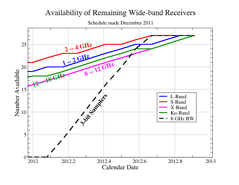
Figure 1: Availability of EVLA antennas and final EVLA receiver systems as a function of time.
It is expected that 8 GHz bandwidth will be made available to all EVLA users in the D-configuration starting in January 2013. New receiver bands will be offered for general use when the performance of at least five antennas has been verified by EVLA commissioning staff.
WIDAR correlator
Overview
Starting with the D-configuration in September 2011 are offering three new OSRO modes. Most striking enhancement is the availability of up to *eight* subbands per baseband instead of just one, thereby increasing the available bandwidth by a factor up to 8.
At the same time we will continue to offer the old 'OSRO 2' mode for those who require the highest possible spectral resolution and don't need the increased bandwidth or a second baseband. Please refer to the description of the OSRO 2 mode on the old OSRO page.
New OSRO modes
For all three new OSRO modes we offer two independently tunable basebands, where each baseband has up to eight subbands. Possible subband widths are 128 MHz, 64 MHz, 32 MHz, all the way down in factors of 2 to 0.03125 MHz. All subbands in both basebands must have the same bandwidth and channelization, and be contiguous in frequency.All three modes offer: full polarization, dual polarization, and single polarization, with 64, 128, and 256 channels per subband, respectively (of course, there is always the possibility during offline processing to smooth in frequency to reduce dataset sizes or to improve spectral response).
- "OSRO: Full polarization": Four polarization products. This configuration will offer 4 polarization products for each sub-band, each of which will have 128 MHz bandwidth with 64 channels. It is possible to decrease the subband bandwidth by powers of two, keeping the same number of channels, to provide the capabilities in Table 1.
Table 1: Correlator capabilities per sub-band for full-polarization
- "OSRO: Dual polarization": Two polarization products. This configuration will offer 2 polarization products for each sub-band, each of which will have 128 MHz bandwidth with 128 channels. It is possible to decrease the subband bandwidth by powers of two, keeping the same number of channels, to provide the capabilities in Table 2.
Table 2: Correlator capabilities per sub-band for dual polarization
- "OSRO: Single polarization": One polarization product (new for OSRO observing). It will offer 1 polarization product for each sub-band, each of which will have 128 MHz bandwidth with 256 channels. It is possible to decrease the subband bandwidth by powers of two, keeping the same number of channels, to provide the capabilities in Table 3.
Table 3: Correlator capabilities per sub-band for single polarization
| Sub-band BW (MHz) | Number of channels/poln product | Channel width (kHz) | Channel width (km/s at 1 GHz) | Total velocity coverage per sub-band (km/s at 1 GHz) |
|---|---|---|---|---|
| 128 | 64 | 2000 | 600/ν(GHz) | 38,400/ν(GHz) |
| 64 | 64 | 1000 | 300 | 19,200 |
| 32 | 64 | 500 | 150 | 9,600 |
| 16 | 64 | 250 | 75 | 4,800 |
| 8 | 64 | 125 | 37.5 | 2,400 |
| 4 | 64 | 62.5 | 19 | 1,200 |
| 2 | 64 | 31.25 | 9.4 | 600 |
| 1 | 64 | 15.625 | 4.7 | 300 |
| 0.5 | 64 | 7.813 | 2.3 | 150 |
| 0.25 | 64 | 3.906 | 1.2 | 75 |
| 0.125 | 64 | 1.953 | 0.59 | 37.5 |
| 0.0625 | 64 | 0.977 | 0.29 | 18.75 |
| 0.03125 | 64 | 0.488 | 0.15 | 9.375 |
| Sub-band BW (MHz) | Number of channels/poln product | Channel width (kHz) | Channel width (km/s at 1 GHz) | Total velocity coverage (km/s at 1 GHz) |
|---|---|---|---|---|
| 128 | 128 | 1000 | 300/ν(GHz) | 38,400/ν(GHz) |
| 64 | 128 | 500 | 150 | 19,200 |
| 32 | 128 | 250 | 75 | 9,600 |
| 16 | 128 | 125 | 37.5 | 4,800 |
| 8 | 128 | 62.5 | 19 | 2,400 |
| 4 | 128 | 31.25 | 9.4 | 1,200 |
| 2 | 128 | 15.625 | 4.7 | 600 |
| 1 | 128 | 7.813 | 2.3 | 300 |
| 0.5 | 128 | 3.906 | 1.2 | 150 |
| 0.25 | 128 | 1.953 | 0.59 | 75 |
| 0.125 | 128 | 0.977 | 0.29 | 37.5 |
| 0.0625 | 128 | 0.488 | 0.15 | 18.75 |
| 0.03125 | 128 | 0.244 | 0.073 | 9.375 |
| Sub-band BW (MHz) | Number of channels/poln product | Channel width (kHz) | Channel width (km/s at 1 GHz) | Total velocity coverage (km/s at 1 GHz) |
|---|---|---|---|---|
| 128 | 256 | 500 | 150/ν(GHz) | 38,400/ν(GHz) |
| 64 | 256 | 250 | 75 | 19,200 |
| 32 | 256 | 125 | 37.5 | 9,600 |
| 16 | 256 | 62.5 | 19 | 4,800 |
| 8 | 256 | 31.25 | 9.4 | 2,400 |
| 4 | 256 | 15.625 | 4.7 | 1,200 |
| 2 | 256 | 7.813 | 2.3 | 600 |
| 1 | 256 | 3.906 | 1.2 | 300 |
| 0.5 | 256 | 1.953 | 0.59 | 150 |
| 0.25 | 256 | 0.977 | 0.29 | 75 |
| 0.125 | 256 | 0.488 | 0.15 | 37.5 |
| 0.0625 | 256 | 0.244 | 0.073 | 18.75 |
| 0.03125 | 256 | 0.122 | 0.037 | 9.375 |
Example: L-band, dual polarization. The two basebands can be tuned independently, e.g. 1250 MHz and 1750 MHz. Each baseband contains 8 sub-bands. The sub-band width is selected from the dual polarization table above, but once chosen, it has to be the same for all sub-bands in both basebands, and the sub-bands have to be contiguous within each baseband. If, say, sub-band width 32 MHz is selected, we have 8 contiguous 32 MHz sub-bands around 1250 MHz (for a total width of 256 MHz) and 8 contiguous 32 MHz wide sub-bands around 1750 MHz (for a total width of 256 MHz). In this example (dual polarization) each sub-band has 128 channels for a 250 kHz channel width throughout.
Constant S/N over many subbands
Due to decreased sensitivity at subband edges, putting together eight adjacent subbands does not result in a constant rms over the total band (see Fig. 2). If constant rms is required, we recommend tuning the two basebands one-half subband width apart. The basebands will largely overlap, but offset from one another by one-half subband width. This causes frequency ranges of decreased sensitivity in one baseband to have nominal sensitivity in the other baseband (see Fig. 3).
There is a price to pay, however, when using this overlapping basebands technique. Without it one can obtain a total bandwidth of 16 times the width of one subband (two non-overlapping basebands of 8 subband widths each). With this technique the total bandwidth is reduced to just 8.5 times the width of one subband.

Figure 2: rms noise in a blank field as a function of frequency for one baseband consisting of 8 contiguous sub-bands. Note the increased rms noise at the subband edges.

Figure 3: rms noise in a blank field as a function of frequency for two basebands consisting of 8 contiguous sub-bands, where the basebands are separated by one-half of the subband width. Wherever signal in one baseband is compromised by edge effects, data from the other subband are substituted.
Other considerations
OSRO capabilities are provided with integration times no shorter than 1 second (for A configuration). For C and D configurations, 5 seconds integration time is the default for L, S, and C band, and 3 seconds for the higher frequency bands. For B configuration the default integration time is 3 seconds, and for A configuration 1 second. Doppler setting to a fixed frequency is supported, but not Doppler tracking. Observers of spectral lines need to make sure their spectral features of interest are at least 4 channels wide, to allow corrections for intra-day frequency shifts to be applied in post-processing while minimizing artifacts due to resampling along the frequency axis. Please consult the Current OSRO Restrictions web page for the most up-to-date information on current OSRO restrictions prior to setting up an observation. Access to the OSRO program will be via the existing time allocation process and regular calls for proposals.
It will be possible to reduce simple OSRO datasets taken in with the correlator configurations described above using either CASA or AIPS.
It should be recognized that the EVLA will be undergoing commissioning throughout the duration of the Early Science programs, and that the quality of data taken during this time cannot be fully guaranteed. Nevertheless, NRAO will make every effort to ensure projects awarded time under the OSRO program do obtain data, subject to the availability of our resources.
Doppler Setting
Description
For spectral line observing, the OSRO modes continue to support Doppler setting (adjusting the observing frequency at the start of the observation to target a particular line: see the Known Issues web page) rather than requiring the PI to periodically submit updated scheduling blocks with new sky frequencies during throughout the configuration.
The ability to have up to eight (contiguous) sub-bands per baseband has the potential to increase the number of lines that are observed at once. Particular attention must be given, however, where the lines of interest will be located within the total baseband, e.g., subband boundaries need to be avoided. The OPT supports this as follows:
- As before, the user specifies the rest frequency that will be used to calculate the required sky frequency.
- New: the user specifies a positive or negative offset (in MHz or in units of sub-band bandwidth) that indicates where the baseband center appears relative to this frequency. Note the following:
- If this offset is 0.0, then the specified rest frequency will be at the center of the baseband, at the boundary/filter edge between two sub-bands (= a bad place!).
- Setting the offset frequency determines in which sub-band the specified rest-frequency will appear.
- Further, if the total bandwidth used is less than 128 MHz, the specified frequency range should be centered in the central 128 MHz filters, i.e., use offsets < 128 MHz to avoid loss of sensitivity when crossing these boundaries.
Example
There are two lines which can be observed based on the required bandwidth and resolution. The two lines are:
- SO2 6(2,4)-7(1,7) at 44052.860 MHz
- CH3OH 3(1,2)-2(2,1) at 44029.320 MHz
Using 4 MHz sub-bands with dual polarization = 128 channels with 31.25 kHz frequency resolution (0.2 km/s at SO2), it is possible to fit these into a single baseband:
- baseband width = 8x4 MHz = 32 MHz
- lines are separated by 23 MHz
The PI specifies the rest frequency of the line of interest: 44052.860 MHz (click to select 'Rest', specify the rest frequency; note this also opens up setting the source characteristics (direction, velocity).
The PI can then specify a positive/negative offset which will be used as the offset from the central frequency:
- Rest Frequency = 44052.860 MHz
- Offset = -13.860 MHz (=approx. 3.5 sub-bands)
This sets the center frequency to 44039 MHz and the full range of frequencies to 44023-44055 MHz (the central frequency specified is at the edge between the 4th and 5th sub-bands); giving:
- 0: 44023-44027 MHz
- 1: 44027-44031 MHz
- 2: 44031-44035 MHz
- 3: 44035-44039 MHz (Note: very center of the baseband (44039 here) is not observable)
- 4: 44039-44043 MHz
- 5: 44043-44047 MHz
- 6: 44047-44051 MHz
- 7: 44051-44055 MHz # Includes SO2 near the middle at 44052.860
Note: Conversion to sky frequencies will happen upon execution; see the top portion of Figure 4.
An example Illustration for the 4-line case with OH at L-band is shown at the bottom of Figure 4.

Figure 4: Illustration of a two-line (top) and four-line (bottom) set-up using Doppler setting for a particular rest frequency and an offset frequency to accommodate additional lines within the observing bandwidths. Blue numbers/black lines highlight the rest frequency and offset frequency used to determine the center of the observing band; dotted lines indicate the 8 sub-band regions. Red lines indicate the 128 MHz filter boundaries within the 1 GHz basebands.

