VLA Calibrator Manual
Phase, Gain, Position, and Polarization Calibration

Coordinate Systems at the VLA
The VLA supports the J2000 coordinate system. Details on this implementation are given by Barry Clark in VLA Computer Memorandum 167 of May 11, 1983. The complete description of the J2000 coordinate system can be found in the USNO circular 163 edited by G. H. Kaplan of the Naval Research Laboratory. See also Johnston et al 1995 (AJ 110, 880). In summary, positions given in the J2000 system will be precessed in accordance with the recommendations of USNO 163. Positions given in the B1950 coordinate system will employ adjustments, so that they are effectively processed by the recommendations of the Explanatory Supplement of 1960. Positions of any other epoch will, currently, be precessed by the recommendations of the Explanatory Supplement of 1960. The most serious consequence of this is that planetary coordinates given in apparent coordinates of observing date are assumed to be in the system of the FK4. It seems likely that as soon as the system of FK5 comes into greater use for the production of planetary ephemerides, we shall reverse this decision, and use the FK5 and the formulae of USNO 163 for epochs other than 1950.
The B1950 system used at the VLA is a bit of an historical oddity. The VLA needed calibrators with accurate positions before the various astrometric (VLBI) lists existed, so they were measured using a reference frame based on a handful of positions (of order 10) from observations with the Green Bank three-element interferometer in 1979.9; those sources were therefore all referred to the B1950 system, epoch 1979.9. When the astrometric lists started coming out from JPL and Goddard, NRAO both added new sources and replaced the old positions with the new, more accurate measurements; these are in the J2000 system, precessed to epoch 2000.0. So the VLA has two fundamental systems: the B1950, epoch 1979.9 frame most natural for the old calibrators, and the J2000, epoch 2000.0 frame most natural for the new ones. In transforming from one frame to the other, e.g. to get a B1950 position for a source originally measured in J2000, both the VLA on-line computers and the OBSERVE program which creates the VLA schedule are "hard-wired" to precess between (B1950, epoch 1979.9) and (J2000, epoch 2000.0). All positions measured at the VLA are in one of these two frames. Just recently positions from the reference frame of Eubanks 1995-1 have been adopted for 475 sources in the calibrator manual, replacing many less accurate positions, and bringing the VLA and VLBA onto the same reference frame.
It now seems profitable for anyone interested in the highest positional accuracy to use J2000 coordinates for all future observations, unless compatibility with previous observations is critical and the whole series does not span enough time to be unduly confused by the known error in Newcomb's precession constant. (It is probably less work to put previous observations in J2000 coordinates than it is to calculate the corrections to the 1950 coordinates of various dates, if the observations span more than a couple of years). For the general VLA user, the pressure to change systems is not so strong--he/she must consider whether it is more important that his observation remain compatible with previous observations of the object, or whether it should be compatible with future accurate astrometry, either radio or optical. We do not recommend changing to J2000 coordinates for an object which you have observed here before, and might conceivably wish to combine the old (u,v) data--there is no point in just asking for trouble. However, we encourage the use of J2000 coordinates for new observations. It seems inevitable that J2000 coordinates are going to come into general use, and the sooner we can get through the painful transition period, the better off we all shall be.
Hints and Strategies for Successful Phase Calibration
In most programs, calibrator sources are observed at least once an hour and sometimes as frequently as every 10 minutes. Calibrator observations are not only important for tracking instrumental phase and gain drifts, atmospheric and ionospheric gain and phase variations, but for monitoring the quality and sensitivity of the data and for spotting the occasional gain and phase jumps.
There are several criteria for choosing and using a calibrator. A list of guidelines, in decreasing order of importance, follows:
- Choose the calibrator closest to your source. If it is within 10 deg., atmospheric phase fluctuations will be somewhat better calibrated. It is better to have one calibrator per source over the entire run. If several are needed, try to bootstrap their positions together. However, in the smaller configurations and at longer wavelengths, these criteria can be considerably relaxed, so a single calibration for a group of sources is often preferable. Furthermore, if your target sources can be self-calibrated, the need for rapid switching between source and calibrator is entirely removed. Hourly observations of the calibrator are more than sufficient for this case, except at 22 GHz or higher frequencies where they should be no further apart than 30 minutes
- Choose a calibrator which has a P or S quality status for the desired configuration and frequency (see Section 4.1). The difference between P and S is minimal but P is preferred since fewer gain errors will result. However, a more nearby but weaker S or even W quality calibrator may well be preferable for phase calibration, but not for amplitude calibration. In this case the amplitude calibration, which is much more stable than the phase calibration, can be derived from observations of a more distant P quality calibrator that is observed less frequently. This situation may arise at high frequencies where only a small number of sources are sufficiently strong (> 0.5 Jy) for amplitude calibration, but the atmospheric phase fluctuations require a nearby calibrator source. As a general rule of thumb, at 0.7 cm the phase calibrator should be within 10 degrees in good weather and within 5 degrees in bad weather. If just solving for the phase, the calibrator can be as weak as twice the sensitivity on a single baseline, which is 0.1 Jy at 43 GHz. If no VLA calibrator is sufficiently close, it may be useful to consult the MERLIN calibrator lists of Patnaik et al. (1992, MNRAS, 254, 655) and Browne et al. (1998; MNRAS, 293, 257). And to properly remove tropospheric phase fluctuations at high frequencies requires very rapid switching with observations of the calibrator every few minutes.
- At frequencies of 1.8 GHz and below, the presence of moderately strong sources within the primary beam centered on the calibrator can cause significant closure errors. For this reason many calibrators have uv restrictions at L and P band and may be completely unsuitable in the smaller configurations. Observations performed in spectral line mode may encounter somewhat larger closure errors than indicated by the P or S quality flags (see the Key in section 4.1) due to the reduction in bandwidth smearing. When observing at L band in the D and C configurations it may be desirable to choose a calibrator with P quality status, even if it is more distant from the target source. Fortunately the atmosphere is quite stable at L band in the D and C configurations.
- Different calibrator codes are used only to distinguish the accuracy of the calibrator position. If absolute positional accuracy < 0.1 arcsec is desired, the position code should be an important consideration - use 'A' or 'B' calibrators. Most positions for sources with 'A' or 'B' PC codes are taken from the JPL or USNO astrometric lists.
- The flux density of the calibrator is of secondary importance. The only exceptions are when the calibrator will be used as a band-pass calibrator for spectral line observing, for high dynamic range observations where closure errors must be measured, and for very narrow-band spectral line experiments.
- The use of partially resolved calibrators for the determination of antenna gains and phases is possible with the added complication that the calibrator must be imaged first and the resulting model provided to CALIB. Use of partially resolved calibrators may occasionally be necessary in the larger configurations. Models are available on the web at http://www.aoc.nrao.edu/~cchandle/cal/cal.html
Planning for Good Polarization Calibration
Introduction
When observing in any of the continuum modes the cross hand products (RL and LR) are produced automatically by the correlator for each IF. Typical "impurities" of the feeds are about 5% for the center of most VLA bands and degrade toward the band edges and away from the pointing center in the image plane. Without any polarization calibration an unpolarized source will appear to be polarized at the ~1% level. Furthermore, without calibration of the R-L phase difference, the polarization angle is undetermined. Fortunately it is not difficult to obtain a reasonably good polarization calibration under most circumstances. With a modest investment of time spent on calibrators and a little effort the instrumental polarization can be reduced to less than 0.1%.
Determining the Leakage Terms (aka D-terms)
The best way to determine the leakage terms (which produce the instrumental polarization), is to observe an unresolved source over a wide range in parallactic angle. The polarization of the calibrator will appear to rotate in the sky with parallactic angle while the instrumental contribution stays constant. The AIPS task PCAL uses this behavior to simultaneously solve for the source polarization properties and the leakage terms. The usual recommendation is for 5 or more observations covering 100 degrees or more of parallactic angle in roughly uniform steps. Strong and compact calibrators (code "P") sources are preferred, although often a reasonably good solution can be obtained from a weaker calibrator observed many times throughout a run for gain and phase calibration. More than one source can be used in the solution provided all sources are unresolved. Algorithms have also been developed in AIPS recently (for VLBI polarization calibration) that allow the use of a single resolved calibrator. In planning an observing run it may be useful to consult the parallactic angle diagram below:
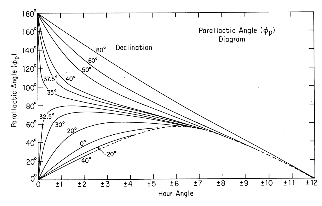
Figure - Parallactic Angle vs. hour angle for various declinations
The leakage terms are also known to be time-variable (Holdaway, Carilli & Owen 1992, VLA test memo #163) and software has been developed in AIPS++ to contend with this variability.
A single observation of a strong unpolarized source (or a source with well known polarization properties) can be used to determine the leakage terms. As an example, 3C84 is strong, unpolarized and unresolved for most VLA frequencies and configurations, so that a single scan on 3C84 may be sufficient. The leakage terms are also fairly constant over weeks to months, so that measurements from one observing run can be passed to another made using the same frequencies and bandwidths and observed in the same configuration. The leakage terms are carried entirely in the antenna table, so to transfer them one merely copies the antenna table.
Calibrating the absolute polarization angles
Calibration of the absolute polarization angle (or R-L phase difference) can be accomplished with a single observation of a polarized source having a known polarization angle (the true R-L phase difference will be twice the source polarization angle). The best source for these purposes is 3C286, which is also a primary flux density calibrator. If 3C286 can't be reached then 3C138 will work in most circumstances. Some information is known about 3C48 and 3C147 as well. All observations of polarization angles summarized below are tied to 3C286 which is assumed to have a Faraday Rotation Measure of 0 rad m$^{-2}$.
| 1995.2 Polarization Measurements | ||||||||||||
| Showing R-L Phase Difference (degrees) and Fractional Polarization (%) | ||||||||||||
| Source | 20cm | 6cm | 3.7cm | 2cm | 1.3cm | 0.7cm | ||||||
| 3C48 | N/A | 0.5 | -148 | 4.1 | -132 | 5.3 | -135 | 7.0 | -145 | 7.6 | -166 | 9.2 |
| 3C138 | -18 | 7.9 | -22 | 11.1 | -22 | 11.9 | -24 | 10.8 | -30 | 10.6 | -23 | 11.6 |
| 3C147 | N/A | <0.1 | N/A | <0.1 | -57 | 0.8 | 110 | 3.1 | 145 | 4.2 | 180 | 5.2 |
| 3C286 | 66 | 9.4 | 66 | 11.0 | 66 | 11.7 | 66 | 12.0 | 66 | 12.0 | 66 | 12.5 |
| 1999.2 Polarization Measurements | ||||||||||||
| Showing R-L Phase Difference (degrees) and Fractional Polarization (%) | ||||||||||||
| Source | 20cm | 6cm | 3.7cm | 2cm | 1.3cm | 0.7cm | ||||||
| 3C48 | -60 | 0.4 | -148 | 4.1 | -138 | 5.6 | -134 | 7.0 | -146 | 8.2 | -172 | 8.8 |
| 3C138 | -15 | 8.0 | -20 | 11.4 | -22 | 11.7 | -24 | 11.7 | -30 | 11.6 | -28 | 12.2 |
| 3C147 | N/A | <0.1 | 16 | 0.4 | -54 | 0.7 | 109 | 2.9 | 147 | 4.5 | 170 | 6.5 |
| 3C286 | 66 | 9.4 | 66 | 11.2 | 66 | 11.6 | 66 | 12.1 | 66 | 12.4 | 66 | 13.3 |
No ionospheric correction has been made to these data, and fluctuations in the ionospheric Faraday rotation, especially approaching the solar maximum in 1999, could cause an error in the above determinations by 10 degrees or more at 20cm. As 3C48 is only weakly polarized at 20cm, it should not be used at this frequency. If it must be used (e.g. no suitable calibrator was observed) then the polarization angle given at epoch 1999.2 can be used. 3C48 may also be undesirable at 22 and 43 GHz where it is weak and variable. At 90cm all the above sources are unpolarized. Some pulsars, however, are strongly polarized and we are investigating using these along with good ionospheric models and data to obtain polarization calibration at 90cm. Contact Rick Perley (rperley@nrao.edu) for further information.
Flux Density Calibration
Accurate Flux Density Bootstrapping
Introduction
Because of source variability, it is impossible to compile an accurate listing of flux densities for most VLA calibrators. The values given in Chapter 4 of this manual are only approximate. We strongly recommend bootstrapping the flux density of a calibrator by comparing the calibrator observations with one or several observations of 3C286, 3C48 or 3C147. Careful observations have allowed the following set of rules to be established for accurate bootstrapping of flux densities using 3C286, 3C48 or 3C147.
3C286 is partially resolved to most combinations of configuration and band. Its resolution occurs on two different scales - there is a weak secondary located 2.5" from the core, and the core itself is partially resolved on longer baselines. Nevertheless, 3C286 can be used as a flux calibrator for all VLA observations providing the rules laid down below are followed.
3C48 and 3C147 are heavily resolved to some combinations of configuration and frequency and exhibit some variability on timescales of months to years (see section 2.2), but nevertheless may be preferable as a flux calibrator over 3C286 since they contain no extended structure on scales greater than 1".
When 3C48, 3C147 and 3C286 can be used directly
The following combinations of array configuration and band have no restrictions in number of antennas or UV range:
| 3C48/3C147 | 90cm | All configurations |
| 20cm | C and D configurations | |
| 6 cm | D configuration | |
| 3.6 cm | D configuration |
| 3C286 | 90cm | B, C, D configurations |
| 20cm | C and D configurations | |
| 6 cm | D configuration | |
| 2 cm | D configuration | |
| 1.3cm | D configuration |
When 3C48 and 3C147 require a model
The following combinations of configuration and band should not be calibrated with 3C48 or 3C147 without supplying a good model.
| 2 cm | A configuration |
| 1.3 cm | A configuration |
| 0.7 cm | A, B configurations |
Some FITS format images, along with clean component models for 3C48 and 3C286 can be found at
http://www.aoc.nrao.edu/~cchandle/cal/cal.html.
http://www.aoc.nrao.edu/~smyers/calibration/
(look for the latest links therein).
If a model is used then no (u,v) restrictions or limitations on the number of antennas are needed. Note that it is still necessary to run SETJY on the primary flux density calibrator even when supplying a model to CALIB.
When special restrictions are necessary for flux calibration
The following rules must be carefully followed to ensure proper flux bootstrapping in the combinations of array scale and band noted below. For the hybrid configurations (BnA, CnB, DnC) the rule for the more compact configuration should be adopted (i.e. follow B config rules for BnA). When specifying inner antennas to be used for the calibration solution, no antenna on the North arm further out than on the East or West arms should be used. Finally, it is a good idea to set WTUV = 0.1 in CALIB to ensure a stable solution.
| Source |
Band (cm) |
uvrange k lambda | config |
number of inner antennas per arm | Notes |
|---|---|---|---|---|---|
| 3C48/3C147 | 90 | 0-40 | All | All | |
| 3C48/3C147 | 20 | 0-40 | A | 7 | |
| 0-40 | B,C,D | All | |||
| 3C48/3C147 | 6 | 0-40 | A | 3 | |
| 0-40 | B,C,D | All | |||
| 3C48/3C147 | 3,6 | 0-40 | A | 2 | |
| 0-40 | B | 6 | |||
| 0-40 | C,D | All | |||
| 3C48/3C147 | 2 | 0-60 | A | 1 | Not recommended |
| 0-60 | B | 5 | |||
| 0-60 | C,D | All | |||
| 3C48/3C147 | 1.3 | 0-80 | A | 1 | Not recommended |
| 0-80 | B | 5 | |||
| 0-80 | C,D | All | |||
| 3C48/3C147 | 0.7 | 0-100 | A | 1,* | Not recommended |
| 0-100 | B | 3,* | See note below | ||
| 0-100 | C,D | All,* | See note below |
| Source |
band (cm) |
uvrange k lambda | Config |
Number of Inner Antennas per arm | Notes |
|---|---|---|---|---|---|
| 3C286 | 90 | 0-18 | A | 7 | |
| 0-18 | B,C,D | All | |||
| 3C286 | 20 | 0-18 | A | 4 | |
| 0-18 | B,C,D | All | |||
| 90-180 | A | All | Reduce flux by 6% | ||
| 3C286 | 6 | 0-25 | A | 1 | Not recommended |
| 0-25 | B | 4 | |||
| 0-25 | C,D | All | |||
| 150-300 | A | All | Reduce flux by 2% | ||
| 3C286 | 3.6 | 50-300 | A | 3 | Reduce flux by 1% |
| 50-300 | B | 7 | Reduce flux by 1% | ||
| 50-300 | C | All | Reduce flux by 1% | ||
| 0-15 | D | All | |||
| 3C286 | 2 | 0-150 | A | 3 | |
| 0-150 | B,C,D | All | |||
| 3C286 | 1.3 | 0-185 | A | 2 | |
| 0-185 | B | 7 | |||
| 0-185 | C,D | All | |||
| 3C286 | 0.7 | 0-300 | A | 2,* | See note below |
| 0-300 | B | 6,* | See note below | ||
| 0-300 | C,D | All |
* NOTE: We are also investigating additional sources that may be suitable as primary flux density calibrators 1.3 and 0.7 cm. The latest information concerning absolute flux calibration at 0.7 cm can be found in the relevant section of the VLA Guide to Observing.
Due to its (u,v) restrictions, low flux density, and evidence suggesting that 3C48 is variable at this wavelength, it is not recommended for flux calibration at 0.7 cm.
If one were to ignore the guidelines, and blindly calibrate the data on the basis of the available data, the flux error obtained would vary according roughly to how much resolution occurs but would not exceed 5% for 3C286. Bear in mind that there will occur a differential error as well, as the antennas at the ends of the array will be over-calibrated with respect to those at the center. If these guidelines are followed, the bootstrap accuracy should be 1 or 2 percent at 20, 6, and 3.6 cm, and perhaps 3 to 5 percent at 2, 1.3 and 0.7 cm. At 2cm and 1.3cm bands, other effects, such as dish efficiency, pointing and atmospheric absorption (1.3cm and 0.7cm) are probably more important.
Elevation-dependent gain corrections
At frequencies of 15 GHz and above, there are appreciable changes in the antenna gains as a function of elevation. Atmospheric opacity, especially at 22 GHz, also introduces an elevation-dependence on the observed visibility amplitudes. By calibrating the target source with a nearby calibrator, much of these variations can be removed. However, if the primary flux calibrator (e.g. 3C286) is observed at a different elevation from the secondary gain and phase calibrator, then the flux bootstrapping will be in error. Proper calibration of the flux densities at high frequencies requires knowledge of a gain curve for the antennas, and the atmospheric opacity as well. Software has been developed in AIPS to address these issues (see the task ELINT). If you don't have enough data to make your own gain curve, you can find gain curves at http://www.aoc.nrao.edu/~smyers/calibration/.
Monitoring of Flux Density Calibrators
Since the planet Mars and 3C295 are too heavily resolved for most VLA observing programs, the flux density of a small set of calibrators is carefully measured with respect to 3C295 and Mars in the 'D' configuration every few years. These more compact sources have been found to be only slowly variable (with some exceptions at the highest frequencies). Below we provide the current (1999.2) best analytic expression for their flux densities.
\[{\rm Log}\: S = A + B \times {\rm Log}\: \nu + C \times ({\rm Log}\: \nu)^2 + D \times ({\rm Log}\: \nu)^3\]
where S is the flux density in Jy and v is the frequency in GHz. These expressions are valid between 300 MHz and 50 GHz.
| Source | A | B | C | D |
|---|---|---|---|---|
| 3C48 | 1.31752 | -0.74090 | -0.16708 | +0.01525 |
| 3C138 | 1.00761 | -0.55629 | -0.11134 | -0.01460 |
| 3C147 | 1.44856 | -0.67252 | -0.21124 | +0.04077 |
| 3C286 | 1.23734 | -0.43276 | -0.14223 | +0.00345 |
| 3C295 | 1.46744 | -0.77350 | -0.25912 | +0.00752 |
The 31DEC99 version (with the proper patch installed) of AIPS program SETJY with OPTYP = 'CALC' will calculate and insert the flux densities based on the above expression and parameters into a VLA database. Alternatively SETJY can be told to use the old Baars et al (1977) expression and parameters (see previous section), or the 1995.2, or 1990 coefficients. AIPS Versions 15OCT89 through 15JAN96 use the 1989.9 coefficients or the Baars coefficients. With versions of AIPS prior to 15OCT89 the flux density of the calibrators must be set with OPTYP = ' ' for each IF. Do not use SETJY with optype 'CALC' if you are switching frequencies within the observing run. In this case you must calculate and insert the appropriate values for each frequency and IF with OPTYP = ' '. You may find it more convenient to split the databases into single FQid components.
Observations taken prior to 1990 may benefit from using the adjustments below when setting the flux density of 3C48, 3C147 or 3C286. Below are listed the RATIOS between the true and Baars et al. value for 3C48, 3C147 and 3C286 at the various frequency bands from 1983 to 1995. Multiply the Baars et al. value by this ratio to obtain the correct flux density. Contact R. Perley or G. Taylor if you need more information.
| 1983.5 | 1985.5 | ||||
|---|---|---|---|---|---|
| L | C | L | C | U | |
| 3C48 | 1.004 | 1.039 | 1.018 | 1.047 | 1.11 |
| 3C147 | 0.974 | 0.957 | 0.970 | 0.948 | 0.99 |
| 3C286 | 0.995 | 1.010 | 0.993 | 1.002 | 0.99 |
| 1987 | 1989.9 | ||||||||
|---|---|---|---|---|---|---|---|---|---|
| P | L | C | X | U | L | C | X | U | |
| 3C48 | 0.95 | 1.02 | 1.04 | 1.06 | 1.10 | 1.019 | 1.043 | 1.049 | 1.076 |
| 3C147 | 1.00 | 0.97 | 0.95 | 0.97 | 1.01 | 0.975 | 0.951 | 0.949 | 0.993 |
| 3C286 | 0.95 | 1.00 | 1.01 | 1.01 | 1.02 | 0.999 | 1.005 | 0.995 | 0.991 |
| 1995.2 | 1999.2 | |||||||||
|---|---|---|---|---|---|---|---|---|---|---|
| P | L | C | X | U | P | L | C | X | U | |
| 3C48 | 0.948 | 1.017 | 1.023 | 1.034 | 1.034 | 0.966 | 1.016 | 1.008 | 1.009 | 1.004 |
| 3C147 | 0.990 | 0.983 | 0.974 | 0.999 | 1.046 | 0.998 | 0.984 | 0.987 | 0.975 | 1.002 |
| 3C286 | 0.971 | 0.999 | 1.008 | 1.006 | 0.988 | 0.967 | 0.999 | 1.008 | 1.007 | 0.989 |
The Flux Density Scale Used at the VLA
The flux density scale used by CASA and AIPS between 1 and 50 GHz is based on the Perley-Butler scale (ApJS, vol 204, 19, 2013). In turn, this scale is based on the absolute Wilkinson Microwave Anisotropy Probe (WMAP) measurements of the brightness of the planet Mars. The corresponding flux densities of Mars were then transferred to four stable calibrator sources (3C123, 3C196, 3C286 and 3C295) through careful VLA measurements of their ratios to Mars spanning more than one decade. The new scale is very close to the traditional Baars et al. (1977 Astron. Astrophys., 61, 99) scale between 1 and 15 GHz.
Below 1 GHz, AIPS and CASA have adopted the 'Scaife and Heald' scale. The VLA has made careful measurements of the ratios of a small set of standard calibrators to Cygnus A, whose absolute flux density is believed to be known to within ~3%. Early results suggest the 'Scaife and Heald' scale is consistent with the known flux density of Cygnus A between 220 and 480 MHz.
VLA Calibrators
Key to the List
Rows
-
Source IAU name at equinox (2000). Use of this name in OBSERVE fetches RA and DEC at equinox 2000 PC Position Code for coordinate accuracy. Position change reference Oct96 Adoption of Eubanks 1995-1 positions from USNO geodetic observations Nov96 G.Taylor A configuration 3.7cm VLA Dec96 C.Carilli A configuration 0.7cm VLA Jan97 G.Taylor B configuration 3.7cm VLA Feb97 G.Taylor B configuration 3.7cm VLA Aug99 M.Goss A config 3.7cm VLA confirmed by 6cm VLA May00 J.Wrobel A configuration 3.7cm and 6cm VLA Dec00 E.Fomalont, VSOP pre-launch survey, 5 GHz geodetic Aug01 VLBA Calibrator Survey astrometric positions Alternate name, if any. The alternate name is NOT recognized by OBSERVE. An entry of CJ2 indicates that the source is included in the Second Caltech-Jodrell Bank VLBI survey, and JVAS is the Jodrell Bank VLA Astrometric Survey. - Source IAU name at equinox (1950). Use of this name in OBSERVE fetches RA and DEC at equinox 1950. Secondary alternate name -- not recognized by OBSERVE.
Position Codes
| A | positional accuracy <0.002 arcseconds |
| B | positional accuracy 0.002 - 0.01 arcseconds |
| C | positional accuracy 0.01 - 0.15 arcseconds |
| T | positional accuracy >0.15 arcseconds |
Notes:
- For the most accuracy J2000 is strongly preferred (see section 3.2.)
- Errors in declination increase in the south, except for A and B calibrators.
Columns
| Column | ||
|---|---|---|
| 1-2 | Band and Band code. For 1.3cm use 2cm entry | |
| 3-6 | Calibrator quality in the A, B, C and D configuration determined using a 50 MHz observing bandwidth: | |
| P | <3% amplitude closure errors expected | |
| S | 3-10% closure errors expected | |
| W | 10-?% closure errors expected. Suitable for calibration of phases only | |
| C | Confused | |
| X | Do not use. Too much resolution or too weak | |
| ? | Structure unknown |
|
| 7 | The approximate flux density of the source. Use only as an indicator of the source strength | |
| 8-9 | CALIB restrictions. These are suggested UVLIMITS in thousands of wavelengths to use in CALIB to avoid data which are contaminated by structure. A UVMIN (Col. 8) generally means the source is confused at short spacings. A UVMAX (Col. 9) generally means the source is resolved at long spacings. Setting WTUV=0.1 in CALIB will help to ensure stability | |
Comments to four calibrators listed below
- Although '?' appears in the table for 0038-213 it is likely that the source is a fine calibrator at 20cm in the A and B configurations since it is unresolved at 6 and 3.6cm at similar resolutions. It is listed with a '?' because we have not confirmed its suitability. Many '?' entries can be interpreted in this way.
- The X at 20cm C and D configurations for 0038-213 and the UVMIN means that the source is confused at short spacings at 20cm. The source could be used, but gain quality would be poorer.
- The source 0714+146 (see below) is only a calibrator at 20cm in the D configuration and in B and C configurations at 90cm. Many similarly extended sources are included in the listings. Most are fairly strong and can be used as bandpass calibrators at 20cm.
- The inaccurate position (PC-T) of 0714+146 is not a restriction for 20cm D configuration observing.
- Note the apparent conflict in UVLIMITS for 1733-130 at 20cm. This conflict is resolved by noting that two different ranges will allow a valid CALIB solution; the first, valid for the D array, is 0 to 3 k wavelengths; the second, valid for the A array, is 40 k wavelengths to the longest baseline (approximately 180 k wavelengths).
- The 2cm listing for 1759+237 has zero flux density and '?' for quality, indicating it has not been observed. Because the source shows a flat spectrum, it is likely to be a good calibrator at 2cm
0038-213   J2000  C 00h38m29.9524s   -21d20'04.027''
0036-216   B1950  C 00h36m00.4390s   -21d36'33.100''
-----------------------------------------------------
BAND        A B C D    FLUX(Jy)    UVMIN(kL)  UVMAX(kL)
=====================================================
 20cm    L  ? ? X X       0.78           10
  6cm    C  S S S S       0.34                      200
3.7cm    X  X S S S       0.22                      200

0714+146   J2000  T 07h14m04.6352s    14d36'20.629''   3C175.1
0711+146   B1950  T 07h11m14.3000s    14d41'33.000''
-----------------------------------------------------
BAND        A B C D    FLUX(Jy)    UVMIN(kL)  UVMAX(kL)
=====================================================
 90cm    P  X S S X          6            1           4
 20cm    L  X X X S       1.90                        4

1733-130   J2000  A 17h33m02.7058s   -13d04'49.546''
1730-130   B1950  A 17h30m13.5352s   -13d02'45.837''
-----------------------------------------------------
BAND        A B C D    FLUX(Jy)    UVMIN(kL)  UVMAX(kL)
=====================================================
 20cm    L  S X X P       5.20           40           3
  6cm    C  P P P P       5.00
3.7cm    X  P P S S       5.80           15
  2cm    U  P P P P       3.70

1759+237   J2000  C 17h59m00.3527s    23d43'46.974''
1756+237   B1950  C 17h56m55.9320s    23d43'55.800''
-----------------------------------------------------
BAND        A B C D    FLUX(Jy)    UVMIN(kL)  UVMAX(kL)
=====================================================
 20cm    L  S S S X       0.70            6          90
  6cm    C  X S S S       1.00                       90
3.7cm    X  S S S S       0.55
  2cm    U  ? ? ? ?       0.00
The List
The focus of this manual is the official List of VLA Calibators. A full description of its entries follows in the next section.
Many of the flux densities reported in the calibrator manual are now over 10 years out-of-date. This means that flux densities reported herein can differ by more than a factor of 2 with current values.
Over the past few years the VLA calibrator manual has continued to grow. A major improvement has been the addition of Q band entries for at total of 1675 calibrators. Note however, that most of the calibrators are flat spectrum and rapidly variable, so the flux densities reported here may not reflect the current level for a given source. Be conservative when selecting calibrators at high frequencies.
In this revision the calibrator manual contains 5523 entries for 1860 sources. Positions for 950 sources were refined on Aug. 28 2001 using the VLBA Calibrator Survey observations as reduced by the NASA Goddard Space Flight Center Geodesy group with the Calc/Solve package. These positions have typical positional errors less than 1 milliarcsec (see Johnston et al 1995, AJ 110, 880; and Beasley et al. 2002, ApJS, 141, 13). This database is also the primary source of positions for the VLBA correlator. We stress that all users who desire accurate positions should use the J2000 coordinates.
The VLA calibrator list has been compiled from many different sources, so it is difficult to assess its completeness. Certainly it is incomplete along the galactic plane, as the majority of the finding lists excluded this region. Not all sources in the list have yet been observed at all bands listed. If no entry exists for a calibrator at the desired frequency the user may still be able to judge its utility based on information given for adjacent bands. This is generally required for selecting K band calibrators. If no suitable calibrator can be found near your target source then you may want to consult the list of other resources for finding calibrators available from the calibrator manual web page.


Connect with NRAO