Guide to Observing with the VLA Complete Manual
Disposition Letter and Scheduling Blocks
Interpreting the Disposition Letter
A disposition letter is sent to the principal investigator and co-investigators of each VLA proposal. This letter contains comments from the cognizant Science Review Panel (SRP), a linear-rank score from the SRP, comments from the NRAO Technical Reviewer and, optionally, comments from the Time Allocation Committee (TAC). Guided by the linear-rank score and taking into account the time available, the TAC assigns a scheduling priority to each session in the proposal. If time is allocated at a scheduling priority of A, B, C or D, the proposal is converted to a project which is eligible to compete for time in the dynamic queue.
The VLA disposition letter is arranged in six portions:
Synopsis This portion lists the proposal id, title, type, authors, cognizant Science Review Panel (SRP), and time allocation summary. The latter tells the proposers whether or not time was allocated to the proposal. If time was allocated, its scheduling priority (A, B, C or D) is given and the proposers are responsible for preparing scheduling blocks for that time.
Comments from the TAC The TAC consists of the chairs of the eight SRPs. Taking into account the time available as a function of LST, the TAC assigns a scheduling priority to each session in each proposal. The TAC might comment on these assignments. The assigned scheduling priority depends on the linear-rank score of the proposal, the LST ranges involved in the session (daytime is harder to accommodate than nighttime), the total time requested in the session, and the competition from better-ranked proposals requesting time at similar LST ranges. For further details, refer to the VLA Prioritizer Memo.
Time Allocation For each session in the proposal, a table lists the session's name, array configuration, time in hours, LST range, bands and scheduling priority. For a given array configuration, time approved at a scheduling priority of A, B, C or D may be divided into multiple scheduling blocks as appropriate. Factors to consider in this division include the scheduling priorities, the observing frequencies, the tabulated LST ranges for the sessions, and the LST pressure plot at the start of the array configuration.
Further information for proposers and observers, including statistics and important LST pressure plots, is available from the most recent TAC report that is referenced in the disposition letter.
The possible scheduling priorities are:
- A = the observations will almost certainly be scheduled
- B = the observations will be scheduled on a best effort basis
- C = the observations will be scheduled as filler
- D = the observations will be scheduled as filler at the lowest priority
- N*= the observations will not be scheduled because they were explicitly rejected by the TAC
- N = the observations will not be scheduled because they could not fit in the time available
Unless otherwise stated in the TAC comments, Regular proposals with: priority B, C and D are eligible for scheduling only in the associated configuration or semester; priority A are automatically carried over for one additional configuration cycle or semester.
Shared Risk Observing (SRO) proposals will not be carried over if they cannot be scheduled for reasons associated with the shared risk component(s) of the observations, even if awarded priority A. Resident Shared Risk Observing (RSRO) proposals are not normally awarded priority A, but would be subject to the same conditions on carry-over as SRO proposals. (See also Re-Observation of FAILED Scheduling Blocks below).
Comments from the SRP This portion gives the linear-rank score from the SRP, along with comments from the SRP that summarize the proposal, give its strengths and weaknesses and, optionally, note any technical issues. The community-based SRP consists of a chair and five anonymous members. The linear-rank score is on a scale from 0 (a high-ranked proposal) to 10 (a low-ranked proposal).
Comments from the NRAO
This section contains instructions for submitting schedule files (see Schedule Creation and Submission below), information about the NRAO Student Observing Support program, and associated deadlines.
Further information for proposers and observers, including statistics and important GST pressure plots, is available from the most recent TAC report that is referenced in the disposition letter.
Comments from the NRAO Technical Reviewer Comments concerning the Technical Justification portion of the proposal, if a technical review has been performed. These comments are available to the SRP and the TAC.
Proceeding with Conversion of Proposal to Project
OVERVIEW
This section discusses converting your proposal to a project, checking the LST pressure plots and how to find the most current version (generated every Friday), scheduling block duration for the different priorities, and some tips on building your scheduling blocks.
Converting a Proposal to a Project
If a proposal's disposition letter indicates that time is allocated at a scheduling priority of A, B, C or D, then NRAO staff will convert the proposal to a project in the Observation Preparation Tool (OPT). This conversion occurs only about a month before the start of an array configuration (see the latest configuration schedule).
After the conversion is complete, the project's authors are notified that the project is ready in the OPT. A project contains one or more program blocks. A given program block will involve only one array configuration (which may be Any) and only one scheduling priority. The project's authors are responsible for atomizing a program block into scheduling blocks.
Interpreting the LST Pressure Plot
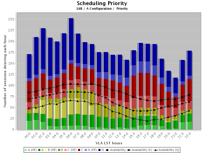
Figure 1.1 (below) shows an example of the pressure on dynamic time as a function of LST for the start of an array configuration; this example is for the A-configuration in Semester 2016B. Similar pressure plots are available for each configuration in each semester and are published in the Time Allocation Committee (TAC) report for the semester.
Figure 1.1 encodes pressure by the scheduling priority assigned by the TAC, as well as by frequencies above 12 GHz (light shading) and below 12 GHz (dark shading). The time available per LST hour is shown by the solid black line for all frequencies, by the long-dashed black line for K-band conditions, and by the short-dashed black line for Q-band conditions. Maintenance, software and enhancement activities cause the thick black line to be less than the total number of LST days in the configuration. Such activities dominantly occur during daytime, causing the black lines to dip for the daytime LST range.
 |
|
Figure 1.1: Example of an LST pressure plot. (Click image for larger view.) |
Scheduling priorities assigned by the TAC are encoded by color, with the following meaning:
- A = the observations will almost certainly be scheduled (light green, dark green)
- B = the observations will be scheduled on a best effort basis (light yellow, dark yellow)
- C & D = the observations will be scheduled as filler (light red, dark red)
- N*, N = the observations will not be scheduled (light blue, dark blue)
A project allocated time at a scheduling priority of A, B, C or D is eligible to compete for time in the dynamic queue. To effectively schedule the VLA, it is necessary to approve more time than is actually available.
Scheduling Block Durations
The duration of an individual scheduling block (SB) cannot exceed the time allocated to its containing program block. Beyond that basic fact, the optimal duration of an SB depends strongly on the scheduling priority (A, B, C or D) assigned to its containing program block. As an aid for observers, a pressure plot for the dynamic queue is updated and posted every Friday, and is accessible from the Schedsoc Home Page.
Priority A: Dynamic scheduling enables priority A SBs to observe during the requested observing conditions, as determined at the start of the observation. SBs of any duration are fine as far as the heuristics in the dynamic scheduler are concerned. However, there may be other considerations in determining the best SB duration. At high frequencies the length of time during which the specified observing conditions, evaluated at the start of the run, can be expected to be satisfied during the duration of the run needs to be considered. This is a function of the time of day and time of year. Daytime observing is also be limited by maintenance, software or enhancement activities, so SBs that can end by 8am or start after 5pm (local Mountain time) have an advantage.
Priority B: The amount of priority B time approved is designed to almost fit into the available hours per configuration. However, it is advantageous to submit SBs of several different durations. SBs with durations of 4 hours, for example, are more efficient, but shorter SBs will often be scheduled earlier, as they can fit around the priority A SBs which are emphasized early in the configuration. Moreover, as noted above, shorter SBs are recommended at high frequencies.
Priority C & D: These are filler projects. Monitor Friday's pressure plot located near the top of the Schedsoc Home Page. Early in the configuration, only SBs with durations of 1 hour or less have any chance of being scheduled. Later in the configuration, SBs with durations of 2 hours or less may be viable. If there are eventually only priority C or D SBs at your LST range(s) of interest, it may be profitable for you to submit SBs with longer durations.
Tips for More Flexible Scheduling Blocks
This section is particularly relevant for SBs with priority C or D, but also for SBs with priority B and involving the most popular LST ranges or the higher frequencies. Some of these tips may also be useful when preparing SBs with priority A.
More flexibility will increase the chance that a particular SB gets observed. However, if the conditions are too flexible or if the overhead becomes so large that the data cannot be calibrated or yields too little time or u-v coverage on the science target, the data set may not achieve the anticipated science goal. Always ensure that the data set can be calibrated. If there are options to consider, it may be better to choose the option that leans toward a more conservative calibration rather than the option that accrues more observing time on the science target. More conservative calibration will also ensure smoother data reduction.
Tips on how to increase the chance that an SB will be observed:
- Submit the SB early. If the SB is not available when a scheduling gap occurs, it cannot be selected for observation. Gaps can occur at any time, including at the planned start of the array configuration (see the configuration schedule).
- Submit a short SB. Short gaps occur more often than long gaps. Make SBs short and repeat them as many times as desired to accumulate observing time. SBs may now have arbitrary lengths.
- Submit SBs with various durations. It is permissible to submit SBs that, in aggregate, exceed the total time allocated to a program block or a project. Use this to your advantage by submitting SBs with various durations. For example, if a scheduling gap of 1.5 hours is available then compete for it with an SB of duration 1.5 hours instead of an SB with a duration of 1.0 hour. That shorter SB can be used to compete for a later scheduling gap of 1.0 hour. Also, as the pressure from priority A and B SBs drops a few months into a principal configuration, scheduling gaps can sometimes accommodate priority C or D SBs longer than 2.0 hours.
- Break up high and low frequency observations. There is more low frequency time than high frequency time, so it is usaully harder to get observed if the weather (API and wind) limits are very low. If it does not matter if low and high frequencies are observed at the same time it is often advantageous to split observations into low and high frequency blocks.
- Relax the API or wind limits for the SB. For example, if the science target is strong enough for self-calibration then the API limit can be relaxed compared to the default value.
- Widen the possible start LST range(s) of the SB. Especially at low frequencies, consider observing down to the elevation limit of the antennas.
Scheduling Block Life Cycle
Project and Program Block Creation
After the approval of a project, the observers are responsible for creating valid Scheduling Blocks (SBs) to achieve their science goals. About one month before the first possible observation, i.e., the start of the requested array configuration in the observing semester, NRAO will create the Project tree with the Program Block (PB) assignments in the Observation Preparation Tool (OPT). Concurrently, the source list is automatically transferred from the Proposal Submission Tool (PST) to the Source Catalog Tool (SCT). If the project consists of observations in more than one array configuration, all PBs will be created at the time of the original import process. Another reminder email will be sent out about a month before observations are anticipated to start in the next array configuration. Once observers have been notified that the OPT has been populated with the Project and PB(s), they may begin creating and submitting valid SBs. Before doing so, it is strongly advised to check whether the import of sources into the SCT have been transferred correctly, e.g., the proper coordinates, epoch, and velocity information (with convention). This is also a good time to create a resource catalog within the Resource Catalog Tool (RCT), also known as the Instrument Configuration tool within the OPT. Once in the OPT, one may also (un)check if an individual on the project would like to receive email notifications for the project, i.e., SB submissions and the operator's observing log emails.
Scheduling Block Creation and Submission
The creation of the SB(s) is the responsibility of the observer(s). The Guide to Observing at the VLA aims to help with this step and contains several suggestions and background information. It is very important for the observer to read through the entire guide, especially the chapter(s) pertaining to their science, e.g., high frequency strategy, low frequency strategy, very low frequency strategy, calibration, polarimetry, spectral line setup, etc. To help observers validate their SB(s) and resource(s), read through the Presubmission Checklists. However, if there is uncertainty regarding the validity of the SB(s), please submit a ticket to the NRAO Helpdesk before submitting the SB(s).
After submission the status of the SB will change from NOT_SUBMITTED to SUBMITTED. The OPT will generate an SB submission email to alert the VLA data analysts to perform a validity check soon thereafter. Note that this is not a science check for, e.g., correct frequencies or spectral line setup, but merely checking the requirements and logistics so it will not disrupt observing. If a submitted SB requires corrections, it can be canceled (unsubmitted), changing the status back to NOT_SUBMITTED.
If the VLA data analysts find any problems with the submitted SB(s), the observer will be notified (preferably through the NRAO Helpdesk) and may be asked to cancel, improve, and/or submit the improved SB(s). Otherwise, when there are no logistical problems apparent, the VLA data analysts will approve the SB(s) for observing, thereby changing the status of the SB(s) to SCHEDULABLE for observing.
At rare occasions, for experienced observers in cases where SBs need to be able to execute very rapidly after submission, e.g., for a target of opportunity, the observers may be given special permission to self-approve their SBs at the time the PBs are created. There will be no validity check of the SB submissions by the VLA data analysts, and the responsibility of the successful execution remains entirely with the observer with the understanding that no make-up time will be granted for unsuccessful observations.
Scheduling Block Observation and Archiving
SBs for observation are drawn from a weighted pool of SCHEDULABLE observing blocks, according to the guidelines explained elsewhere in this guide. When an iteration of an SB gets queued, a copy is created known as an Execution Block (EB). The EB lives as QUEUED, RUNNING, PENDING FAILURE or PENDING COMPLETION before the final EB status of FAILED or COMPLETED. Note that these short-lived intermediate EB status designations are merely helpful to the operators and staff. After the successful execution (observation) of each iteration of the SB, the observer will be notified of the successful completion of an iteration of the SB. The status of the SB will remain SCHEDULABLE as long as there are remaining iterations. The successful completion of all repeat-iterations specified in the SB will mark the status of the SB as COMPLETED. The observer can retrieve the individual SB executions of the data from the NRAO data archive. Data will be proprietary to the original observers typically for one year after the last observation taken for the project; after which the data becomes public and accessible to all archive users.
Occasionally, mostly for logistical reasons, during the scheduling of observations in the dynamic scheduling process, the operator may defer an SB to ON HOLD. This is a very short-term status and the operator or NRAO staff will quickly release the SB back to the queue or take other actions to resolve any issues. In some cases, for miscellaneous reasons, the execution of an SB may not complete. Scheduling blocks with an EB having a status of FAILED will be investigated and, if appropriate, the observer will be contacted for follow up. An SB with a FAILED execution block typically triggers a re-observation at a later time (see also Re-Observation of FAILED Scheduling Blocks below).
Scheduling blocks that have not been observed, or have remaining repeat iterations at the end of the observing period allocated to the project (typically at the end of the allocated array configuration(s) or observing semester), will be given the status of EXPIRED and will be removed from the active observing queue. Once COMPLETED or EXPIRED, the SB becomes read-only and thus cannot be unsubmitted or edited. However, the SB can be read and (partially) copied to a new SB in a new or otherwise active PB which can then be modified for new observations.
Scheduling Block Status Monitoring
Observers who have switched on their email notifications in the Project will receive emails for each SB of the project when the status changes to SUBMITTED, or back to NOT_SUBMITTED. Currently, we are working on a notification when a SB becomes SCHEDULABLE or EXPIRED.
Anyone on the project can monitor the status of the SBs in the project by logging into the OPT. The status summary of all SBs in a program block (PB) is viewed by selecting the PB level of the Project tree. Here the number of anticipated executions (or counts), LST start range, and the wind and API constraints are listed. For each execution of an SB, including repeat executions, the PB level of a Project contains a table of Execution Blocks (EBs) listing the corresponding SB ID, status, duration, start and finish date/time (in LST and UTC), initial API and wind readings (which are likely to change during the observation) can be found below the table of SBs. The same information can be found under the Executions tab within an SB. This information is added after an SB is executed, and the corresponding EB is created.
Observers may monitor a webpage setup to display a list of what has been observing on the VLA for the last 12 hours (updates every 10 minutes).
Re-Observation of FAILED Scheduling Blocks
Occasionally, an observation will fail for any of a number of possible reasons. If a project is in the General Observing category, it will be placed back into the dynamic queue for possible re-observation when conditions allow. Those projects in the Shared Risk and Resident Shared Risk categories may not be re-observed if they fail due to problems with the shared risk/resident shared risk component(s) of the observation. If observers believe that an observation should be failed after inspecting their data they should submit a ticket to the NRAO Helpdesk as soon as possible and in all cases prior to the expiry of the period of eligibility for scheduling.
Dynamic Scheduling Considerations
Introduction to Dynamic Scheduling
Most scheduling blocks (SBs) are observed dynamically, based on factors that NRAO controls and on factors that the observer controls. Such dynamic scheduling enhances science data quality and the array's ability to discharge time-sensitive science. On rare occasions, an SB that requires coordinated observations with other telescopes will be scheduled on a fixed sidereal date. If you have questions regarding the scheduling of your SBs please contact the VLA schedulers via email at schedsoc@nrao.edu or via the NRAO Science Helpdesk using the VLA Scheduling Support department.
NRAO staff use the Observation Scheduling Tool (OST) to examine the current observing conditions and the queue of SBs submitted for the current array configuration. The observing conditions are quantified by the RMS phase measured with the Atmospheric Phase Interferometer (API), the wind speed, and the sunrise/sunset time. The OST then applies heuristics to create a schedule, which is just a time series of optimal SBs. The first optimal SB in the series is then sent off for execution by the monitor and control system. Just before that execution completes, the OST again applies heuristics to create a new schedule.
The heuristics used by the OST include the scheduling priority (A, B, C or D) assigned by the Time Allocation Committee or Director's Discretionary Time Committee and, for TAC reviewed proposal, the linear-rank score assigned by the Science Review Panel. The heuristics also include SB attributes under observer control, specifically its duration, weather constraints (API and wind limits), observing bands, range of LST start times and, optionally, an earliest start date and a request to avoid sunrise/sunset.
Dynamic scheduling obviously means that the observer does not know when the observations will occur. This must be kept in mind when preparing an SB. In particular, the observer should check that none of the possible LST start times create problems with antenna wraps and the scans of the flux density scale calibrator. These topics are discussed in more detail below.
Doppler Correction
For some spectral line setups, Doppler correction (position and velocity) should be applied. The benefit of Doppler Setting, since the VLA is dynamically scheduled, is that it calculates the sky frequency at the beginning of an SB and keeps this fixed for the duration of the SB. Doppler Setting can be specified for each individual baseband in the OPT, removing the burden to do this for each possible observing run by the observer. For more details, refer to the Doppler Correction section within the Spectral Line guide.
Antenna Shadowing
An antenna is shadowed when its line-of-sight to the source is partially or fully blocked by another antenna in front of it. The shadowed antenna will collect less radiation from the source than if it had not been shadowed, reducing the sensitivity on the baselines to that antenna. Shadowing is more likely to occur when sources are at low elevation and when the antennas are in more compact configurations. The OPT will report, per scan, the maximum amount of shadowing, if any, will occur according to the location in the sky of the target and the configuration of the observations. D-configuration is affected by shadowing more than the other configurations because the antennas are at their closest proximity to each other. If you select "Any" configuration, the OPT will calculate the worst-case scenario by assuming the D-configuration to calculate shadowing.
If any calibration scans will be shadowed for any of the valid LST start times, we recommend increasing the observing time of the calibration source to account for the loss of sensitivity. Table 2.3.1 shows the amount of shadowing in respect to the fraction of an antenna that is blocked with the corresponding loss of sensitivity. All shadowed baselines will be similarly affected. Note that the loss of sensitivity is not linear with the fractional shadowing.
| Shadowing | Fraction of Area Blocked | Baseline Sensitivity Loss |
|---|---|---|
| 1 m | 0.01 | 0.5% |
| 5 m | 0.10 | 5% |
| 12.5 m | 0.39 | 22% |
| 18 m | 0.64 | 40% |
| 25 m | 1 | 100% |
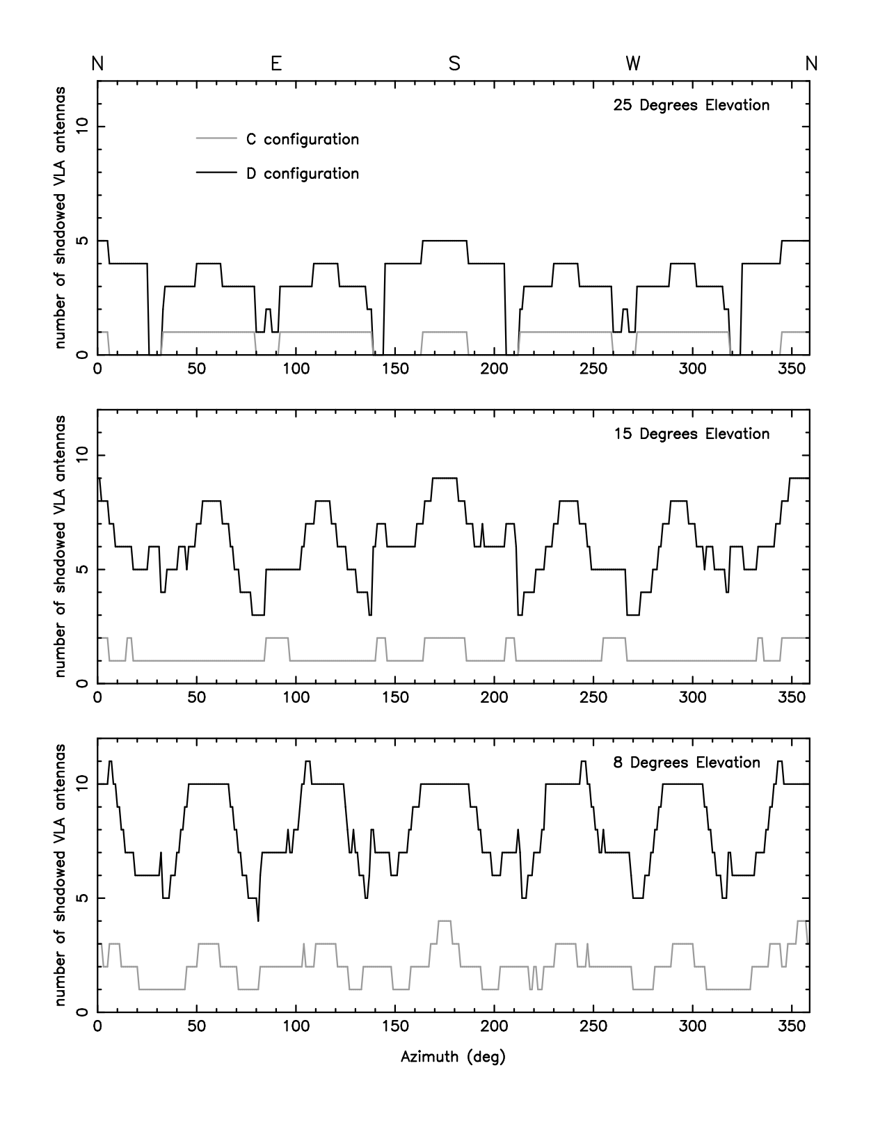
Avoiding antenna shadowing during the D-configuration relies on the azimuth of the antennas, which is dependent on the location of the source and the LST start time. Therefore, to guarantee no more than a single shadowed antenna, restrict the elevations, if possible, to >40° for D-configuration and >25° for C-configuration. Shadowing is worst along the azimuths of the arms (in both directions), so has a six-fold symmetry. See Figure 2.3.1 below. Note that the maximum elevation (in degrees) for your target is its Declination plus 56°, so it may not be possible to avoid any shadowing for sources at Dec < -16° or Dec < -31° for D and C configuration, respectively.
 |
|
Figure 2.3.1: Plot of shadowed azimuths in D-configuration (black line) and C-configuration (grey line), for three elevations: 25°, 15°, and 8°. (Important note, these plots and the post processing packages (AIPS and CASA) do not calculate shadowing flags for an antenna placed on the Master Pad or the antenna barn.) |
Antenna Wraps
Before we dive into the details of antenna wraps, the OPT will now recommend an LST start range based on selected elevations (minimum and maximum limits) for a Scheduling Block (SB) containing all appropriate scans, including, but not limited to, science target(s), complex gain calibrator, flux density scale calibrator, etc.. The recommended LST start range(s) may also include suggested antenna wrap requests. For more details, refer to the following sections under the OPT manual: Create an SB and Scans and Dynamic LST Validation Tab.
- Tip: The suggested antenna wrap per LST start range should be double checked by selecting the wrap on the first few scans (roughly the first 10min) and then check the SB on the Static Report tab and the Dynamic LST Validation tab. In most cases, only one wrap should be used per LST start range. For example, if the OPT recommends two LST start ranges with opposite antenna wraps, we recommend making a copy of the SB to make use of each LST start range and corresponding antenna wrap. If you do not want both SBs to run, you may link them so only one is observed while the other is expired. Refer to the OPT manual on how to link SBs.
Introduction
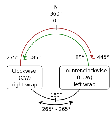
To help avoid confusion, we will define some terminology. For a visualization of these terms, refer to the wrap diagram below (Figure 2.4.1).
| Wrap Type | Definitions |
|---|---|
|
Clockwise (CW) Right or Outer |
When looking down at the VLA from above, the antennas on a CW wrap would appear to be tracking in azimuth in a CW direction from 180° real Az. |
|
Counter-clockwise (CCW) Left or Inner |
When looking down at the VLA from above, the antennas on a CCW wrap would appear to be tracking in azimuth in a CCW direction from 180° real Az. |
| North | This term is used where the CW and CCW wraps overlap between 275° and 85° real Az, passing through 0° / 360° (north) (CW: 275° to 445° (85° real Az) / CCW: −85° (275° real Az) to 85°). |
| South | This term is used for the unambiguous section of the wraps where there is no preference over the use of either CW or CCW wraps. The south wrap is from 85° to 275° real Az, passing through 180° (south). |
During the observation of a single source, or by switching from one source to the next, the antennas are continuously changing their pointing toward different directions in the sky. The cables for power, communication, and data transfer have a limited length and wrap around the rotation (azimuth) axis of the antenna while the antenna moves. Software directs the antenna movements to prevent them from tightening and snapping when the cables reach the azimuth cable wrap limit, i.e., when they have wrapped ±265° either direction (CW or CCW) from the south (at 180° real azimuth). At a wrap limit, instead of continuous tracking during a scan or directly moving to the next scan at a scan boundary, the antennas will move the opposite long way while unwrapping the cables. As the azimuth slew rate is 40°/min, a full 360° azimuth unwrap will take up 9 minutes (plus some settling time) of unusable observing time (this can vary slightly per antenna). It is important to avoid such a situation and pay attention to the antenna azimuth and wrap during the observation, which means paying attention to the wrap when the azimuth of the scan in the Schedule Summary reports if the scans approach 85° and 445°, or when the scan sequence crosses −85° and 275° azimuth (see Figure 2.4.1 below). Perhaps experiment with different azimuth (and elevation) starting positions to investigate the effect (and starting slew times) for a particular scheduling block (SB).
Another inconvenient wrapping situation appears when observations near zenith (elevations larger than about 80°) switch between sources on different azimuth wraps. This happens when a target and calibrator are close to, but on opposite sides of 34.1° (34°04′43.497′′) Declination (latitude of the VLA). The OPT will show slew times much longer than expected for the angular source separation, and indicate an azimuth wrap (CW or CCW) on only one of the sources in the reports of the scan list. So even if a calibrator may be a bit further away or less strong, it may be the better option when it is on the same side of zenith. Experiment with different LST start times to investigate the effect for a particular SB if no suitable calibrator can be found on the same side of zenith.
The most important antenna wrap issue arises at the start of the SB as the wrap chosen determines the wrap for the rest of the observation (if not specified in further scans). This wrap should also align the azimuth of antennas combined from previous different subarrays at the start of observing. At the end of the previous program the antennas (or subarrays of antennas) are left pointing in a direction that is dependent on the previous program, and may be any azimuth between −85° and +445°. When the antennas slew toward the first source in the SB, there are two options: clockwise (CW, also known as Right or Outer) or counterclockwise (CCW, also known as Left or Inner); see Figure 2.4.1. In dynamic scheduling, the software will choose the shortest slew to the first source unless otherwise specified in the antenna wrap option in the first scan(s) in the SB. This default software choice may or may not be the optimum case for the observations. To avoid problems, if any of the scans in the SB are observed outside the range between +85° and +275° in the south, then specify the antenna wrap at the start-up sequence (roughly the first 10min) to be assured that thereafter the wraps in the reports listing correspond to the actual wraps during the observations. Only when all scans in the SB remain between, or completely avoid the range of +85° and +275° azimuth during any of the start times specified in the LST start range, there is no explicit need to specify any wrap. That is, observations entirely on the south wrap or entirely on the north wrap should be fine, but if you include any of the common standard flux density scale calibrators (i.e., 3C48 or 3C286) most likely the observation will include LSTs where these sources are on the other wrap.
Summary of Wraps
When to request an antenna wrap: Unless the first source (i.e., setup scan(s) and the first standard observing or reference pointing scan) is always in the unambiguous (south) part of the wrap (85° ≥ Az ≤ 275°; see Figure 2.4.1 below) during any LST start time within the set range, then you should request an antenna wrap for each scan of the start-up sequence (generally the first 10–15 minutes of the SB). If the SB starts with either 3C286 or 3C48, then an antenna wrap should be selected and continue to specify that wrap for the startup sequence of the SB. Be aware that when 3C286 or 3C48 rise and set they cross the ambiguous (275° ≥ Az ≤ 85°; see Figure 2.4.1 below) part of the wrap, which can cause problems with unwrapping to the next source (i.e., the complex gain calibrator), so there may not be any time on the first complex gain calibrator scan or the first science target scan.
Which antenna wrap to choose: Look at the first scan under the Schedule Summary report to check if there is an unwrap issue (275° ≥ Az ≤ 85°) for all times in the LST start range. Follow how the azimuth evolves during the observing block and whether it crosses the 275°/85° boundaries. Select a wrap which takes the antennas in a direction so there is plenty of room for the antennas to move without having to unwrap again; check the LST start range by stepping through at least every hour, making sure that all scans have plenty of on source time (no less than 20sec for standard observing and no less than 2min30sec for reference pointing). Sometimes the LST start range will need to be adjusted to avoid an unwrap.
Antenna Wrap Caveats: When the schedule summary reports a calculated wrap CW or calculated wrap CCW, do not assume that the calculated wrap will be the starting wrap. The calculated wrap is also a good indication that a wrap should be set, but not always in the calculated direction.
Addressing Both Wraps: When an SB can have two LST start ranges to cover the rising and setting of sources, we recommend submitting two SBs to cover the two LST start ranges and their corresponding antenna wraps. For more details on how to create linked SBs, refer to the FAQs page or the Linking SBs section of the OPT manual.
Antenna Wrap Bugs in the OPT:
- In some circumstances, and only for the first and second scan, there is a discrepancy in the reporting of the telescope azimuth. This is apparent when an SB starts on a source that is always in the north (Dec > 34°) using the default of azimuth 225° (i.e., in the south). In this case, the OPT may report a confusing starting azimuth on the first scan and an azimuth jump and/or a wrap change for the second scan (even if it is the same source). This bug can be ignored and no wrap need be set.
- A slightly different wrap display bug in the Reports page, is where the first and second scan on the north wrap may differ by 360°.
Detailed Guide
Wrap Diagram
Figure 2.4.1 shows the antenna wrap diagram; this diagram is very helpful in resolving wrap issues. Use this diagram in conjunction with the azimuth column in the scan listing of the Schedule Summary Report table for different LST start times to investigate whether any wrap issues may occur. Often wrap issues will appear when the standard flux density scale calibrator sources 3C286 and 3C48 are scheduled to be observed at rise and/or set at either limit of the LST start range, or when they might be observed during culmination at zenith. That is, many observers should take note to avoid any problems by adhering to the antenna wrap guidelines.
It should be noted, for completeness, that the online software monitors the azimuth of the antennas constantly (i.e., on time scales of seconds; not per scan). As soon as the actual azimuth of a particular antenna hits the −85° or +445° azimuth limit, the antenna will be directed to unwrap and slew in the opposite direction to catch up with the observation instruction. As this happens at the actual azimuth (after the global pointing model and possible additional reference pointing corrections are applied), the time at which a specific (the first) antenna might unwrap may be different from another antenna (the last) by a minute or so. To avoid unwrapping antennas at different times, make sure the scans do not start or stop very close to these azimuth limits for any of the potential LST start times of the SB.
|
West |
 |
East |
| Figure 2.4.1: VLA wrap diagram with Azimuth conventions and readings and the cable wrap limits. Clockwise wrap goes over West (red; outermost curve from the bottom to the top of the spiral) and Counterclockwise over East (green; innermost curve). South (unambiguous) wrap is between azimuth +85° and +275° (black; bottom of the spiral) and North (ambiguous) wrap is in the area at the top, between −85° and +85° or +275° and +445°. | ||
Antenna Wrap & Elevation Considerations
A source is rising when the LST (modulus 24h) is less than the RA of the source. A source is setting when the LST is greater than the RA of the source. Note that for this reasoning, the RA and LST (range) should be within 12h of each other to properly determine rise or set. If the difference is larger, add 24h to either the RA or LST range values, whichever has the lower value in the SB.
- If all of your sources, targets, and calibrators have Declinations below about 8.5°, they are all observed in the south wrap and will never reach the ambiguous wrap region: no wrap setting is needed. Note that this almost never happens as you want to include one of your flux density scale calibrators and all have a Declination larger than 8.5°. If any of the sources has a Declination very close to 8–9°, this rule of thumb may not apply and more care should be taken in checking the observing schedule. This 8.5° limit assumes observations all the way down to the elevation limit of 8°. For observations using higher elevation limits, the 8.5° Declination rule becomes a higher-than-nine Declination rule, depending on the actual elevation limit:
|
|
Elevation limit |
8° | 10° | 15° | 20° | 25° | 35° | 45° | 60° | 90° |
l=latitude (34o04' for VLA) |
|---|---|---|---|---|---|---|---|---|---|---|---|
| Highest Dec. on the south wrap (Az=85°), i.e. never on north wrap | +8°35' | +9°41' | +12°24' | +15°02' | +17°35' | +22°21' | +26°34' | +31°25' | +34°04' | sin(d)=sin(l)sin(e)+cos(l)cos(a)cos(e) or for VLA approximately sin(d)=0.5602*sin(e)+0.0722*cos(e) | |
| Lowest observable Dec. (Az=180° south) | -48° | -46° | -41° | -36° | -31° | -21° | -11° | +4° | +34° |
d=e+l-90, or for VLA d=e-55o56' |
|
| Circumpolar Declination (on north wrap) | +64° | +66° | +71° | +78° | +81° | (+90°) | d=e+90-l, or for VLA d=e+55o56' | ||||
- If all of your sources (targets and calibrators) have Declinations above about 34°, they are all observed in the north wrap and will never use the south wrap region: no wrap setting is needed. Note that this is unlikely unless you use 3C147 as your flux density scale calibrator or 3C295 (in the case you observe only below 2 GHz in D configuration). If any of the sources has a Declination very close to 34°, this rule of thumb may not apply and more care should be taken in checking the observing schedule.
- If your first source has a Declination of less than about 34° and is rising at the start of the observation, set the starting sequence wraps (first 10–15 minutes worth of scans at the start of the block) to CCW (left). If the first source is setting, set the wrap to CW (right).
- If your first source has a Declination of more than about 34° (i.e., it will be observed in the north), then there are two options that will only make a difference once the next source in the sequence has a Declination below about 34° (otherwise you can use the second rule above). If that next southern Declination source at the time of the observing LST (i.e., the starting LST time plus the duration of time into the observation) is rising then set the starting sequence (first 10–15 minute worth of scans at the start of the block) wraps to CCW (left). If this southern source is setting, set the beginning sequence wraps to CW (right).
Always make sure to check the wraps in the Reports tab of the SB in the OPT. If in doubt or confused, please leave the wrap designation to "No Preference" and consult the NRAO Helpdesk.
For more detailed information on setting antenna wraps, see the section How to Proceed below.
Wrap Issues & Standard Flux Density Scale Calibrators
The default standard flux density scale calibrators for the VLA, 3C286 (J1331+3030) and 3C48 (J0137+3309), are nicely separated by about 12 hours in Right Ascension (RA) but, unfortunately, have two major inconveniences. First, their Declination is almost the latitude of the VLA (34.1°), which causes them to culminate almost at zenith on the southern wrap and, second, while they are mostly in the southern wrap, they rise and set in the northern wrap. Catching these flux density scale calibrators in short SBs may be difficult for target observations in certain regions distant from these calibrators on the sky. Therefore, it quite often happens that the flux density scale calibrator is observed in these dynamic SBs when a flux density scale calibrator just rises or just sets, where wrap issues may become a problem for targets on the southern wrap. For targets on the northern wrap, even though the flux density scale calibrators may be high in the sky, it decreases the usable LST start range to place the flux density scale calibration scans if wrap issues are to be avoided. See Table 2.4.2 and Figure 2.4.2 for details.
Table 2.4.2: Wraps and wrap limits for Standard Flux Density Scale Calibrators at the VLA
| North Wrap | South Wrap | North Wrap | ||||||
|---|---|---|---|---|---|---|---|---|
| Rise at | Az= 85/445° | Az= −85/275° | Set at | |||||
| Az | LST | LST | El | El | LST | LST | Az | |
| 3C48† | 55/415° | 18:42 | 23:53 | 68° | 68° | 03:23 | 08:33 | −56/304° |
| 3C286 | 59/419° | 06:45 | 10:53 | 57° | 57° | 16:09 | 20:18 | −58/302° |
| 3C138* |
75/435° | 23:16 | 00:29 | 23° | 23° | 10:13 | 11:27 | −75/285° |
† 3C48 has varied in flux density over the last few years, but appears to have settled down.
* The flux density scale calibrator 3C138 is currently undergoing a flare. As of January 2025, the change in flux density is greater than 10% at all frequencies greater than 4 GHz (i.e., C-band). At present, the magnitude of the flare is approximately a factor of 2 at K-band, 3 at Ka-band, and 4 at Q-band. Monthly monitoring observations are available for investigators that require an accurate flux density scale when using 3C138. These observations are publicly available in the archive under the project code TCAL0009. A table of scaling factors per band per month from February 2021 onward has been provided.
| Rise at | Easternmost Azimuth |
Westerenmost Azimuth |
Set at | |||
|---|---|---|---|---|---|---|
| Az | LST | LST | Az | |||
| 3C147 | 33/393° | 21:32 | 51/411° | −51/309° | 13:53 | −33/327° |
| 3C295‡ | 30/390° | 05:45 | 48/408° | −48/312° | 22:38 | −30/330° |
‡ Disclaimer: CASA does not have a flux density scale model for 3C295.
 |
|
Figure 2.4.2: Antenna wrap a a function of LST for the standard flux density scale calibrators. (Click image for a larger view.) |
When the source is observed at an LST shown in green in Figure 2.4.2 (above), the source is in the south and typically no wrap issues arise. When the LST is red, the source is in the northern wrap and either a CCW (left; at rise) or a CW (right; at set) wrap should be specified in the scan. For 3C147 and 3C295 the wrap should be specified as well; the wrap, however, will depend on the efficiency to reach the other sources specified in the schedule. The yellow LST regions are when the sources, 3C48 and 3C286, are at an elevation above 80° and should probably be avoided during high frequency observing. (Note, low frequency observing can observe up to 85° in elevation, too much higher in elevation can cause antenna wrap issues.)
How to Proceed
Initially, it is best not to worry about the antenna wrap until the SB has been created. Then extensively check the azimuth of the scans in the SB for all LST start times in the anticipated LST start time range. This action will reveal if any wrap issues occur for some or all of the possible LST start times.
Aside from any wrapping issues, remember that 3C286 and 3C48 culminate near zenith. To avoid pointing problems at high elevations (≥ 80°) during high frequency observations, it is probably best to avoid having scans for these flux density scale calibrators during the LST range 12:47–14:15 for 3C286 and the range 00:50–02:25 for 3C48. Restrict the LST start range so the scans with 3C286 and/or 3C48 will not happen for these LST times, or perhaps even split the LST start range in two (or more) non-overlapping LST start ranges in the INFORMATION tab of the SB. Ideally, one would want to observe the flux density scale calibrator at about the same elevation as the target sources to obtain a more accurate flux density, especially at the higher frequencies. However, this is hard to plan and not always manageable with dynamic scheduling: it would require a restricted LST start range which would decrease observing chances. Another suggestion, for similar reasons, is to try and observe the flux density or bandpass calibrator when the target source passes through zenith (if its Declination is near 34°).
Assuming that the target sources are not scattered all over the sky (e.g., for a survey), there are essentially four cases when using 3C286, 3C48, and/or 3C138:
- 3C286/3C48 can only be observed between rise and culmination in the (South)East: The target source is leading the flux density scale calibrator in the south or north of zenith, typically by up to 6 hours in RA (otherwise the other flux density scale calibrator is more likely to be chosen).
- For Dec < 34.1° the target source will be south of zenith and set after the flux density scale calibrator rises. There should be no wrap issues if the wrap directs the antennas to observe the flux density scale calibrator in the CCW (left) wrap or when the LST start range is limited such that the flux density scale calibrator scan can only happen after the LST time for Az = 85°/445° for that flux calibrator in the table above. Typically, the flux density scale calibrator is observed at the end of the SB.
- For Dec > 34.1° the target source will be north of zenith and stay on the north wrap. There should be no wrap issues if the flux density scale calibrator is observed before the LST time for Az = 85°/445° for that flux density scale calibrator in the table above. Typically the flux density scale calibrator is observed whenever the scan can fit in the LST range for the eastern north wrap, i.e., between rise time LST and the LST time for Az = 85°/445° for that flux density scale calibrator in the table above.
- 3C286/3C48 can only be observed between culmination in the (South)West and set: The target source is trailing the flux density scale calibrator in the south or north of zenith, typically by up to 6 hours in RA (otherwise the other flux density scale calibrator is more likely to be chosen).
- For Dec < 34.1° the target source will be south of zenith and rise before the flux density scale calibrator sets. There should be no wrap issues if the wrap directs the antennas to observe the flux density scale calibrator in the clockwise CW (right) wrap or when the LST start range is limited such that the flux density scale calibrator scan can only happen before the LST time for Az = −85°/275° for that flux density scale calibrator in the table above. Typically, the flux density scale calibrator is observed at the start of the SB.
- For Dec > 34.1° the target source will be north of zenith and stay on the north wrap. There should be no wrap issues if the flux density scale calibrator is observed after the LST time for Az = −85°/275° for that flux density scale calibrator in the table above. Typically the flux density scale calibrator is observed whenever the scan can fit in the LST range for the western north wrap, i.e., between the LST time for Az = −85°/275° and set time LST for that flux density scale calibrator in the table above.
- 3C286/3C48 can be observed throughout the SB duration for all LST start times: For this case one would probably choose whether to put the flux density scale calibrator close to the start or close to the end of the SB. Placing it in the middle would not minimize the chances of culminating during the SB and introduce wrapping issues for northern wrap target sources. By placing the flux density scale calibrator observations at the start or the end of the SB, either of the above cases would apply as guideline on how to proceed. Continue checking the azimuth for different LST start times and perhaps even change the strategy on where to place the flux density scale calibrator observations.
- More complicated than any of the three above: If the SB cannot be converted to a simpler case by grouping source scans to the same wrap and/or choosing the flux density scale calibration scans at the start or end of the SB, this case may become more like a trial-and-error approach. Usually this is not a problem; however, if it remains, continue checking the azimuth for different LST start times, maybe limit the LST start range even further and/or perhaps even change the strategy on where to place the flux density scale calibrator observations.
After creating the SB, please check the wraps and look out for possible issues for all possible LST start times in the LST start range before submitting the SB. This may be time consuming but will prevent surprises during observing and in the data. When setting a wrap at the start of the SB, please continue to specify the same wrap during the start-up sequence, i.e., for all the scans that make up the first 10–15 minutes for the SB to force it to be effective.
Note that the slew to the first source, and the calculated wrap it chooses is calculated from the assumed starting position as specified in the INFORMATION tab of the SB. By default, this starting position is pointing toward the south; but the actual starting position is from wherever the previous program has left the antennas pointing (anywhere from azimuth −85° to +445°), and not necessarily the same direction for each antenna. Playing around with the starting azimuth may help to determine the maximum slew time for the worst case scenario and whether different wraps are possible for different LST start times. For testing maximum slew times at the start of the observation the worst cases arise, with the wraps specified as suggested above:
- When one or more antennas are at Az = −85° and the SB is started at the latest possible LST start time of the LST start range, and;
- When one or more antennas are at Az = +445° and the SB is started at the earliest possible LST start time of the LST start range.
For high frequency observations, there should be at least 2min30sec on source time in the reference pointing scan in addition to the worst case slew time. And to complicate it even further, the worst pointing case may not be at the worst starting LST.
Please ask the NRAO Helpdesk if you need assistance.
Avoiding the Sun
The Sun is a bright and variable radio source and can be a problem for VLA observations at all frequencies if it is near the target source. Phase fluctuations and elevated system temperatures will result when observing too close to the Sun. This section gives guidelines on how far sources should be from the Sun as a function of observing band at the VLA, as well as some links to tools to help in planning observations. Please note that these guidelines should not be confused with avoiding daytime observing for RFI reasons, or avoiding sunrise and sunset for phase stability reasons.
Currently, the OPT does not look for or flag SBs containing sources which could be observed too close to the Sun. The Observation Scheduling Tool (OST) will provide a Sun proximity message to the VLA operators to note in the observing log. However, this does not mean the operator will not proceed with a non-solar observation if the sources are too close or behind the Sun. It is the responsibility of the observer, to monitor both if and when their sources will be too close to the Sun and the activity of the Sun. The VLA Sun & Moon Distance Check Tool can help determine if and when a source will be too close to the Sun. This tool also gives the distance to the Moon, although typically the Moon is not a problem unless it is very nearby (within a few primary beam FWHMs).
Solar Activity Webpages
- NOAA Space Weather
- Long Wavelength Array (LWA) provides near real-time and archival solar activity (< 100) MHz all-sky observations.
Handling SBs with Sources Near the Sun
If any of the sources in an SB are too near the Sun (especially if it is particularly active), then there are a couple ways observers may address this:
- On the Information tab of an SB, you may set an earliest/latest UT start date/time to avoid dates when the sources will be too near the Sun. This field can be edited at any time, i.e., before/after SB submission and when the SB is schedulable (in the observing queue).
- You may also unsubmit the SB. If you choose to unsubmit, please be sure to resubmit when appropriate. We will not know why the SB was unsubmitted and will not preemptively re-submit when solar activity has subsided.
Recommended Observing Distances from the Sun
Table 2.5.1 shows the minimum distance from the Sun for 10° phase errors (Φ), assuming the longest baselines can be tolerated. Depending on the solar activity of the Sun, the acceptable observing distance will increase.
Note: We have noticed an increase of solar activity causing problems with phases in the data. Consider a more conservative distance from the Sun than what is list in the table. For example, L-band in D and C-configuration may want to consider observing ~10-20° from the Sun.
The numbers in table 2.5.1 were calculated via:
\[R_{deg}≈\left(\frac{7\lambda_{cm} * B^{0.29}_{km}}{\phi_{deg}}\right)^{0.71}\]
where Bkm is the baseline in km, λcm is the frequency in cm, and Φdeg is the phase error in degrees. Details on how this equation was derived are in VLA Test Memo 236, "How close to the Sun should we observe with the VLA?" Another useful memo is EVLA Memo 136, "EVLA Measurements Close to the Sun: Elevated System Temperatures."
More details about the effect of the Sun on VLA observations may be found in the Low Frequency and Very Low Frequency strategy guides.
| Rdeg | |||||
|---|---|---|---|---|---|
| Band | λcm |
A (36km) |
B (11km) |
C (3km) |
D (1km) |
| Q | 0.7 | 3° | 3° | 3° | 3° |
| Ka | 1.0 | 3° | 3° | 3° | 3° |
| K | 1.3 | 3° | 3° | 3° | 3° |
| Ku | 2.0 | 3° | 3° | 3° | 3° |
| X | 3.5 | 4° | 3° | 3° | 3° |
| C | 6.2 | 6° | 5° | 4° | 3° |
| S | 10 | 8.3° | 7° | 5° | 4° |
| L | 21 | 14° | 11° | 8° | 7° |
| P | 90 | 40° | 31° | 30° | 30° |
| Table 2.4: Short distances have been rounded up to 3°; distances less than this should always be avoided. P-band at C and D-configurations have been rounded up to 30° to minimize the impact of the Sun on these observations. Therefore, distances less than these should always cause concern, and greater distances may be required depending on the observation and the activity of the Sun. | |||||
Weather Constraints
The Observation Scheduling Tool (OST, aka, dynamic scheduler) uses the current Atmospheric Phase Interferometer (API) and wind speed, as well as the predicted wind speed when deciding whether to run an observation, i.e., a Scheduling Block (SB). If the API, current or future wind speeds are above the constraints set in the SB using the OPT then the SB will not be selected. This can make it difficult to observe high frequency SBs.
Wind Limits
The wind speed limit is based on the fact that wind will push the VLA dishes around causing the primary beam to move on the sky. At higher frequencies the primary beam is smaller and so it is easier to move a dish enough to move the target out of the center of the primary beam, therefore the wind speed limit is lower at higher frequencies. Wind speeds higher than the limits will cause the amplitudes to vary which cannot be calibrated after the observation.
Atmospheric Phase Limits
The recommended API limits are based on estimates of the maximum API limit assuming that the science target could not or should not be self-calibrated. If the science target can be self-calibrated then the API limit can be much higher giving the SB a greater chance to be observed. Starting in December 2022 there are two possible Atmospheric Phase Limits (APLs) to choose from depending on whether or not the science target can be self-calibrated.
The following table lists the default weather constraints available in the Observation Preparation Tool (OPT) for each observing band. An observer may choose between the conservative APL or the less conservative self-calibration APL. The wind limit will remain the same between either APL choice.
|
Observing Band |
Wind (m/s) |
Conservative APL (degrees) |
|
Self-calibration APL (degrees) |
| 4, P, L | Any | Any | Any | |
| S | Any | 60 | or | 120 |
| C | Any | 45 | or | 90 |
| X | 15 | 30 | or | 60 |
| Ku | 10 | 15 | or | 30 |
| K | 7 | 10 | or | 20 |
| Ka | 6 | 7 | or | 14 |
| Q | 5 | 5 | or | 10 |
How to Choose the APL for Your SB
Choose the lower (conservative) limit if:
- The science target is too faint to self-cal (see below), or
- The flux density of the science target is unknown and likely faint, or
- There is a scientific reason not to self-calibrate, e.g., when the scientific goal is to perform astrometry
Choose the higher (self-calibration) limit if:
- It is desirable to self-calibrate the science target, and
- The signal to noise ratio (SNR) of the science target is > 3 in a solution interval using the subband width (for continuum) or the anticipated line/channel width (for spectral line) for a single baseline and polarization.
- a solution interval (solint) should be based on how fast the atmospheric phases are likely to be changing and therefore shorter for higher frequencies and longer baselines.
- for a 25 antenna VLA the SNR of the target peak flux density/rmssolint should be ≥20
Examples
- Example 1: The science target is a compact source with a peak flux density of 15mJy/beam. Observing occurs in A-configuration at Ka band continuum. Should we use the higher APL?
- Estimate the solint. The recommended calibration cycle time for A-configuration and Ka band is 3 minutes so we assume that the atmospheric phases will vary faster than that with the higher APL (which allows for observations at less favorable weather during the observation). So let's pick a solint of 30 seconds, which would allow ~6 solutions over 3 minutes to track the variations.
- Determine the rms for 30 seconds and a bandwidth of 128MHz, a single polarization and 25 antennas in Ka band using the VLA Exposure Calculator.
rmssolint=0.48mJy/beam - Calculate the SNR: SNR=15/0.48=31 (peak/rms, all in mJy/beam)
As this ratio is over 20, this source is good to self-calibrate and therefore one can use the higher APL - Example 2: The science target is a maser line in K band with a line width of ~3km/s (~220kHz). The expected peak flux of the maser is 147mJy over 3km/s or in a ~220 kHz channel and the observation occurs in C-configuration.
- Estimate the solint. The recommended calibration cycle time for C-configuration and K band is 6 minutes so we assume that the atmospheric phases will vary faster than that with the higher APL. So let's pick a solint of 1 minute, which would allow ~6 solutions over 6 minutes to track the variations.
- Determine the rms for 1 minute and a bandwidth of 3km/s or ~220 kHz, a single polarization and 25 antennas in K band using the VLA Exposure Calculator.
rmssolint=10.5mJy/beam - Calculate the SNR: SNR=147/10.5=14 (peak/rms, all in mJy/beam)
This ratio is not near 20 so this maser source is probably not a good source to self-calibrate; use the lower, more restrictive APL.
Caveats
- The theoretical rmssolint might be lower than the actual image rms for many reasons (e.g. RFI, overhead unaccounted for) and therefore self-calibration could be difficult. The SNR ≥ 20 is a slight overestimate of the SNR needed because of the likelihood that the rms will be slightly higher than that given by the VLA Exposure Calculator.
- If the target is dominated by extended emission, the flux detected by longer baselines may be much lower than the peak. It then might be difficult to get good self-calibration solutions on the longer baselines, although uv-restrictions in the self-calibration procedure may help.
- The recommendations and examples above are conservative. There are tricks that can be used to self-calibrate in non-ideal situations. If you are an experienced user and you know you can self-calibrate your science target then please use the higher APL; in that case doing these calculations can be skipped.
Good luck with your observations!

Calibration
This section discusses general calibration and calibration strategies when preparing for VLA observations. Specific calibration during post-processing—not depending on data taken during the observations—such as improved antenna positions, opacity and ionospheric corrections, are not discussed here. Note, however, that there is specific guidance with respect to the 8/3-Bit Attenuation and Setup Scans that are required in observing scripts (scheduling blocks).
If you are looking for the listing of VLA calibrators, go to the VLA Calibrator List. This list may also be searched in the Source Catalog Tool (SCT, aka Sources). The OPT manual has a section on how to search in the SCT.
Calibration Basics
What is calibration?
The main goal of calibration is to be able to correct for effects that may interfere with the scientific outcome of a measurement (an observation) due to the instrument and/or local temporary conditions so that these measurements can be compared to other measurements (at other times, other instruments, other frequencies, etc.) and theoretical predictions.
Calibration starts in the device design stage and ends in the final data presentation. Calibration can refer not only to calibration of the data, but also to the instrument as a whole or its separate components. The amount of calibration typically depends on the observing program and the science goal. Some calibrations need to be done once as their solution is fairly constant over time, while other calibrations need to be repeated regularly to capture changing properties over time. For radio astronomy, and in particular interferometry, the following general calibration steps can be identified: calibration of the instrument by observatory staff, calibration of the current observing conditions by the observer, and calibration of scientific results by the data analyzer. Some common calibration examples:
- Calibration of the antenna (receiver frequencies, receiver system temperatures, optics), antenna positions, timing, and correlator visibilities is done by observatory staff.
- Calibration of instrumental delay, instrumental polarization, spectral bandpass response, absolute flux density scale, and other possible properties—assumed to be constant during the observation—should be taken by the observer, typically once or twice during the entire observation for each observed frequency and correlator configuration.
- Calibration of antenna pointing, delay, attenuator and requantizer settings, and other possible properties assumed to be only slowly varying during the observation should be performed by the observer, typically once every hour or so during the observation, or, for example, when switching frequency bands.
- Calibration of antenna gains, atmospheric phase fluctuations, and other possible properties expected to vary more rapidly with observing conditions and geometry during the observation should be performed more frequently than the time scale over which the property changes.
- Calibration of the position of a source with respect to another source, calibration of a frequency to a line-of-sight velocity, calibration of a polarization angle to a reference angle, calibration of the flux density scale of a single source in one observation to another observation of the same source, etc.
The taking of calibration data to be evaluated in the online system or in post-processing happens before, during, and after the observation and also may be applied before, during, and after the observation. Note that most calibration applied before and during the observation, e.g., antenna pointing, take effect during the observation and the calibration must be correct as it cannot be adjusted after acquisition.
It should be understood that calibration is an important part of the observation and must be thoughtfully included in the observation preparation and time request in the proposal. The key point of planning and including calibration is that if the observations are not properly calibrated, the science goal will not be achieved.
When to calibrate?
Calibration should be performed, at the very least, more frequently than the time scale over which the property changes and before that change becomes too large to be compensated for. Nearly constant properties should be calibrated at the start of an observation, when changes from a previous observation by another observer are to be expected. If the constant property can be applied in post-processing, this calibration can also be taken at the end of the observation. Time or geometry dependent changes should be monitored at regular intervals so that the change can unambiguously be interpolated over the observation. Planned, abrupt changes in the observation, such as a frequency change or observing a different part of the sky, would trigger calibration. Last, but not least, a very specific science goal may need a calibration that is not among the standard calibrations described here. The calibration strategy is the responsibility of the observer, but NRAO staff is available for individual advice through the NRAO Helpdesk.
Typical calibration intervals are once during the observation for flux density, bandpass/delay, and polarization angle (per frequency setting and per correlator configuration). It is prudent to at least break up the flux density calibration scan into two or more separate scans, as this is the only calibration for which there is no good alternative if it happens to be corrupted.
Typical intervals for complex gain (amplitude and phase) calibration are dependent on the weather conditions and baseline length. On longer baselines (i.e., on longer uv-distances and therefore more important for high frequency observing), the phase change on the interferometer will be more rapid and requires more frequent calibration than at the lower observing frequencies. An exception at low frequencies is when the Sun affects the ionosphere and rapid changes can be expected near sunset and sunrise. Otherwise, the largest effect on phase change is in the troposphere. The gain calibration uses the assumption that the calibration toward the sky, in which the calibrator source is observed, can be interpolated over time and viewing angle and resembles the same atmospheric conditions toward the sky of the target source. The further away the calibrator from the target, and the longer the intervals of the calibration measurement, the less strict this assumption will hold. It can happen that calibration consumes more than half of the allocated observing time in order to achieve the scientific goal. Fortunately, this may only be necessary at the highest frequencies, in the largest array configurations, and in bad weather conditions. With the introduction of dynamic scheduling at the VLA, this latter variable has been largely eliminated and gain calibration has been easier to plan (see below).
Typical calibration intervals for attenuator settings are at the beginning of an observation. Requantizer gains need to be redetermined after a change of tuning, including when returning to the original observational setup.
Calibration intervals for antenna pointing are largely dependent on the geometry of the observation. As a rule-of-thumb, after tracking for about an hour, the direction of the solutions of the antenna pointing calibration will have changed significantly from where the target position is now—on the order of 20°—warranting a new pointing solution. During the day, because of temperature changes that affect antenna optics, pointing should be repeated roughly every 30 to 40 minutes. Also, when slewing a large distance from the target to a flux density or a bandpass calibrator (over 20° in AZ and/or EL), the antenna pointing will need an updated solution.
How to calibrate?
To ensure that the instrument is delivering the expected measure, the easiest method of calibration is to insert a known signal at the input and analyze the resulting signal at the output. The calibration measurement will yield, after some massaging, the corrections that need to be applied to the output signal to obtain the true representation of the input signal. The uncorrected output signal is also known as the instrumental response for the given input signal. As determining the response directly is not always possible, alternatives may be available. These alternatives require, however, certain trade-offs and choices to be made by the observer depending on the science goals. Observatory staff can advise, and a first attempt is made below. For very specific questions, please ask the NRAO Helpdesk.
A typical calibration signal for the instrumental response of an individual antenna signal path is a pulse (the firing of a noise diode in the receiver) and standard instrumental calibration procedures are available. A typical calibration signal for the total observational response of an interferometer is to observe a point source: a signal that can be considered a simple, single, isolated object with a known constant flux density, polarization as function of frequency, and absolute sky position. As these objects are very rare for high-angular resolution and high-sensitivity interferometers like the VLA, alternatives that dominate the response (not necessarily constant in flux density) and that are near point-like are common trade-offs for any radio interferometer. Many of these calibrator sources are given in the VLA Calibrator List.
Then, depending on the signal property to calibrate, one would choose an adequate calibrator source for the property and insert it at the appropriate place in the observing schedule. This calibration is defined for a certain point in time for certain conditions and needs to be redone when it starts to become invalid. Performing a calibration on the target field—a field where obtaining the measured properties are the goal of the observation—generally is not a good idea. As a reasonable approximation in general, therefore, it is assumed that for the calibration performed near in time and near that field on the sky also holds for the target field and thus can be interpolated over the target observation. NRAO tries to provide guidance for when these assumptions hold for different sets of observations, but the observer should always be aware that certain conditions for successful interpolation of calibration may not apply.
Specific suggestions for different VLA calibrations and how to schedule them are listed elsewhere in the Guide to Observing (High Frequency Strategy, Low Frequency Strategy, and Very Low Frequency Strategy), and the OPT Manual. In this section the focus is on general, non-frequency specific, calibration during the observation by the observer. When making a schedule, consider the hints given here and elsewhere in the documentation. Do not hesitate to contact the NRAO Helpdesk for assistance or further information.
VLA Calibration by the Observer
When seen from the observer's perspective, for any standard observation in each scheduling block, the observer is expected to include calibration of the absolute (flux density) scale, calibration of the signals at different frequencies relative to each other over the observing bandwidth (bandpass), and calibration of the time dependent effects (complex gain (phase and amplitude)) of changing conditions due to the atmosphere and instrument. More sophisticated or challenging experiments may include more specific calibrations as described below.
Flux Density Scale Calibration
The correlator, where signals at specific frequencies from the antennas are combined into visibilities, only processes what it gets fed from the electronics system in terms of relative signal strength and relative phase. The correlator products, therefore, need to be readjusted to represent the flux density as measured from the sky visibilities. At the VLA this means that one observes a calibrator with a postulated (or assumed) known flux density at these frequencies along with the other observations in the scheduling block. In post-processing, the visibilities are then rescaled for this calibrator to the flux density for this frequency. Other visibilities in the same observation, using the same setup, can simply be matched using the relative scale and the absolute flux density of the calibrator.
The flux density scale adopted for the VLA between 1 and 50 GHz is based on the Perley and Butler (2017) standard. This is very close to the traditional Baars et al. scale (1977 A&A 61, 99) between 1 and 15 GHz and includes the Scaife and Heald scale (2012, MNRAS 423, L30) for frequencies below 1 GHz. Distributed versions of AIPS and CASA apply the most recent scale in their SETJY tasks.
Because of source variability, it is impossible to compile an accurate and up to date listing of flux densities for all the VLA calibrators. The values given in the VLA Calibrator List, therefore, are only approximate and for the epoch they were measured. We strongly recommend, and some science objectives require, bootstrapping the flux density of a calibrator by comparing the calibrator observations with one or several observations of 3C286, 3C48, 3C147, or 3C138**. Only in compact configurations and at low frequencies, i.e., typically at L- and P-band in C and D configuration, 3C295 or 3C196 may also be used. However, CASA does not have a flux density scale model for 3C295 or 3C196.
Both AIPS and CASA use model images for the standard flux density calibration sources (see their respective SETJY documentation) to account for their structures which are frequency and array configuration dependent. Alternatively, u,v restrictions, or limitations on the number of antennas, can be used. When using models, the bootstrap accuracy should be within a couple to a few percent. However, at frequencies of about 15 GHz and above, there are appreciable changes in the antenna gains and atmospheric opacity as a function of elevation. By calibrating the target source with a nearby calibrator, much of these variations can be removed. If the flux density scale calibrator (e.g., 3C286) is observed at a different elevation from the complex gain calibrator, however, then the flux density bootstrapping will have a considerable systematic error. For the higher frequencies, a typical discrepancy in actual versus measured flux density scale of the order of 20-30% is not unlikely.
Accurate models are available in both AIPS and CASA for various frequency bands for the calibrators 3C286, 3C48, 3C147, and 3C138**. However, neither 3C295 nor 3C196 has such models and the VLA CASA calibration pipeline will fail if these two calibrators are used. Also, the bright source 3C84 (J0319+4130, not to be confused with 3C48) cannot be used as an absolute flux density calibrator as it is variable, but it serves well for bandpass and delay calibration.
See also the flux density scale discussion in the VLA Observational Status Summary (OSS).
** The flux density scale calibrator 3C138 is currently undergoing a flare. As of January 2025, the change in flux density is greater than 10% at all frequencies greater than 4 GHz (i.e., C-band). At present, the magnitude of the flare is approximately a factor of 2 at K-band, 3 at Ka-band, and 4 at Q-band. Monthly monitoring observations are available for investigators that require an accurate flux density scale when using 3C138. These observations are publicly available in the archive under the project code TCAL0009. A table of scaling factors per band per month from February 2021 onward has been provided.
Bandpass and Delay Calibration
Small impurities in the correlator model, such as an inaccurate antenna position, timing, etc., cause small deviations from the model that are noticeable as a time-constant linear phase slope as function of frequency in the correlated data for a single baseline. This phase slope, known as a delay, is a property of the IF baseband and the same for all subbands (spectral windows) in a baseband. If the frequencies in an observation are averaged into a continuum image, an uncorrected delay causes decorrelation of the continuum signal and is not a correct representation of the sky. The delay calibration is determined on a short time interval on a strong source in order to achieve high signal to noise for the solution without including the time dependent variations.
Small impurities in the frequency amplitude and phase response as function of frequency, independent of the delay, also occur and have to be corrected. These corrections are a property of the passband on top of the response of the baseband, and are a property of the subband and the location of the subband in a baseband. Leaving the bandpass uncorrected causes incorrect relative amplitudes and phases and does not deliver the correct spectral representation of the sky. Averaging these uncorrected impurities over frequency into a continuum image limits the achievable signal to noise and dynamic range. As for the delay, bandpass calibration is usually determined on a short time interval on a strong source to achieve high signal to noise for the solution without including the time dependent variations. Delay and bandpass calibration, therefore, is usually performed using the same calibrator. Hereafter in the text, delay calibration is implicitly included in the bandpass calibrator or bandpass calibration scan.
To achieve good results in both spectral line and continuum observations, the baseband delay and subband bandpass shapes have to be calibrated for each frequency setup. If very high dynamic range is not the aim (in many cases for continuum observations, the standard flux density calibrators are relatively convenient bandpass and delay calibrators), using flux density calibrators has the big advantage that, for these sources, the known spectral index can be included in the bandpass amplitude solution. At high frequencies, however, for which the flux density calibrators are weak, other calibrators might provide a better alternative.
The typical requirement for bandpass calibration is that it does not add to the phase or amplitude noise in the image cube, i.e, that the signal to noise of the bandpass calibration solution is comparable—or better—than the signal to noise of the flux density of the target. The requirements, however, are dependent on your science goals and type of observation. For very bright spectral lines on the order of tens of Jy in a single spectral channel, this might not be feasible; for other spectral line cases it is a good rule of thumb. As the noise is proportional to the inverse of the root of bandwidth times observing time, and with the channel bandwidth a constant between the scans, the time spent on the bandpass calibrator (tcal) should be larger than the time spent on the target (tobj) multiplied by the square of the ratio of the target (Sobj) over the flux density calibrator (Scal): tcal > tobj × (Sobj / Scal)2. That is, the brighter the calibrator, the shorter the scan needs to be. Note that instead of a bright bandpass calibrator, it is also possible to sum all scans of a gain calibrator to obtain sufficient signal to noise for a bandpass determination. For plain continuum observations this requirement can be somewhat relaxed to a good solution of a representation of the bandpass, as the data are averaged over frequency, using a minimum signal to noise at least 5 to approximately 10. If one is interested in high dynamic range or accurate polarization imaging, however, this solution typically is not enough and one would have to adopt the spectral line approach.
The Spectral Line guide describes more details. For further information or other questions contact the NRAO Helpdesk.
Complex Gain Calibration
Where the absolute flux density scale calibration is a static multiplier, and the bandpass/delay calibration a one-off determination of the signal path properties assumed to be largely constant for the observation, the antenna gain calibration (also known as complex gain) is anticipated to track time variable properties due to changing conditions of the instrument. Complex gain calibration also tracks changes with the environment except for antenna pointing (see below), that, if not corrected for, will be absorbed. Examples of variable instrumental properties are: receiver power level settings, corruption of baseband samplers, technicians removing receivers, etc.. The largest time variable contribution is from the environment and atmosphere: mostly the ionosphere at low frequencies, the troposphere at high frequencies, water content/opacity on cloudy days, elevation/opacity due to observing geometry and other occasional phenomena like solar flares, broadcasting satellites, tourist cell phones, digital cameras, etc. Some of these can be calibrated and corrected for using proper gain calibration while others, referred to as Radio Frequency Interference (RFI), cannot and need to be removed (flagged) from the data.
Gain calibration is normally considered antenna based and assumes that fluctuations in the antenna gain are due to slowly varying amplitudes and phases. Slowly here means that the interval of the gain calibration scans are short enough that the variations can be interpolated by a relative smooth function which would represent the true variation at the antenna. Gain phase varies much, much faster than gain amplitude as most of the time dependent effects affect phase more than amplitude. Additionally, phase variations scale with baseline length with more rapid changes on longer projected baselines. The typical time for such changes to become large enough to require calibration is referred to as the coherence time, i.e., when the visibility phase has changed by a radian. This coherence time may be some tens of minutes at short baselines and low frequencies or, in some realistic cases, sub-minute on long baselines for high frequency observations in non-optimal weather. Because of this huge range and frequency specific dependence, consult the Cycle Time section at the end of this document.
Gain calibration is performed as regularly repeated scans on the complex gain calibrator to measure the change in visibility amplitude and phase on the gain calibrator. These changes are then interpolated over the target field scan. Removing the large fluctuations, in effect, increases the coherence time of the observation; ultimately to longer than the total target observation duration. All data on the target field scan can then be coherently combined into a single image, which supposedly would be the goal of the observation. Note that the calibration solutions sometimes show deviant points with respect to the solutions of other times for the same antenna. Recall that these are the solutions (or corrections) needed to obtain the point-like input signal and are not necessarily wrong. It is a good indication that something is happening in the data and, only upon investigation, should one decide whether or not using that point in the interpolation to the target field. That is, will it improve or destroy the target data, or be irrelevant in the case of self-calibration (see below)? The discrepant solution can be deleted to prevent interpolation and thus causes target data flagging, or be kept for subsequent calibration and imaging.
Calibration can be considered for three different cases:
- To only capture the slowly varying amplitude fluctuations. The coherence time to track and interpolate phase over the target field is irrelevant because the target field contains sufficiently bright emission to recover the phase fluctuations on time scales shorter than the coherence time. Typical cases are a targeted, not necessarily point-like, strong continuum source; a bright maser line at any observing band; or, e.g., the background continuum field for the large field of view (primary beam) of the lower frequency bands. As the information to perform this phase calibration (next to the amplitude gain calibration) is contained in the target field, this additional target field calibration is known as self-calibration or selfcal. Care should be taken in the self-calibration model as, in principle, absolute phase—and therefore absolute position—is lost in the process.
- To capture the rapid phase variations in addition to the amplitude variations. Here it is attempted to extend the effective coherence time as self-calibration is not an option for faint targets or detection experiments. Also, very extended or complicated source structures, when a selfcal model is not easily obtained, are typical cases for this traditional gain calibration strategy where the calibrator and target are observed in alternating scans. The target field phases are tied or referenced to those of the calibrator, which is known as phase referencing. The cycle times for alternating the scans are dependent on observing frequency, baseline length, field separation, weather, and elevation. Suggested times are given in table 4.3.1 (below), where cycle times are discussed. If, after such calibration, it appears that the target field matches the requirements for self-calibration, then self-calibration may be applied to further improve the calibration.
- To obtain astrometry. For this one should avoid applying selfcal and utilize a much more careful phase calibration scheme. Some hints on phase-referencing for astrometry are given below.
Specialized Calibration
Antenna Reference Pointing Calibration
When directed to a position in the sky, the individual antennas are commanded to move in azimuth (AZ) and elevation (EL) until they report that they have arrived. The a priori accuracy of pointing at the actual position in the sky is typically within about 10 arcseconds; but individual antennas may differ up to an arcminute in AZ and/or EL. and the deviation depends on many non-constant factors. At the higher frequencies (above ~15 GHz), this intrinsic pointing error may be a large fraction of the primary beam (which is one arcminute at 45 GHz, two arcminutes at 22 GHz, etc.), potentially considerably degrading the sensitivity of the antenna at the position of interest. It is therefore important to correct for this possible mechanical error before observing the calibrators (complex gain, bandpass, etc.) and the target field. Antenna pointing calibration is essential for high-frequency observing but, as the beam sizes at lower frequencies quickly become many arcminutes, pointing calibration is typically skipped for the lower frequencies. One exception is high-dynamic range imaging of large fields where differing antenna beam patterns on the sky will hinder obtaining accurate source flux densities in the entire field of view and pointing calibration also at low frequencies may be imperative.
Simple procedures, referred to as reference pointing, are in place to determine the AZ and EL position offsets during the observing program using X-band. Once determined, these offsets should be applied to the scans following to take effect immediately; this is an on-line calibration. Pointing calibration sources (see about choosing one below) can be your default calibrator sources (for flux density, bandpass and/or complex gain), as well as your target source if your science goal and target source would allow that. A pointing calibration scan needs an on-source time of 2m30s to be able to perform a five-point observation around the calibrator to derive solutions.
The antenna pointing offset will change after some time due to changes in the dish structure (optics) or because the target field is being tracked from rise in the East to set in the West. The reference pointing solution needs to be repeated before the pointing has degraded to yield less sensitivity. NRAO recommends that pointing be repeated when the difference from the last pointing calibration direction in AZ or EL coordinate has changed by 20° on the sky, i.e., after about an hour when tracking a source at the celestial equator assuming nighttime observing. During daytime observing reference pointing may need to be repeated every 30-40 minutes due to the thermal deformation of the dish structure. The recommendation noted earlier also implies that the pointing calibrator source should be closer than that range from the target field; NRAO recommends that the pointing calibrator be within of 10° of the target if at all possible. Hence, large slews to a bandpass or a flux density calibrator, or a different target patch on the sky, will require a new pointing scan regardless of how long it has been since the last one was done.
Polarization Calibration
The VLA observes with two orthogonal receivers. These are right and left circular polarization (RCP and LCP) for all bands except below 1 GHz where they are X and Y linear polarization. For the total intensity Stokes parameter I, the correlator produces the parallel hand correlations (RR and LL or XX and YY) from the signals of the two antennas of each interferometer. They are combined in the imaging to produce the total intensity I image of the sky; Stokes V may be created from the RCP and LCP difference. Using the default continuum modes, the cross hand polarization products (RL and LR or XY and YX) are also produced which allow to map the other Stokes parameters Q and U and combine all data into an image of the polarized sky.
In order to obtain the correct polarization characteristics, two calibrations have to be performed. First, because the receivers are independent and orthogonal but not completely free of impurity, the leakage (D-term) and relative signal between the receivers as function of frequency need to be determined in order to properly combine the signals (compare it with the frequency dependence of amplitude and phase over a bandpass). The polarization vectors should then be tied to an absolute reference with a polarization angle calibration (compare it with fixing the absolute flux density) using a source with known polarization characteristics, like 3C286.
Typical impurities of the receiver feeds are a few percent for the center of most VLA bands and degrade toward the band edges and away from the pointing center in the image plane. Without any polarization calibration, an unpolarized source will appear to be polarized at a few percent level. Without calibration of the R-L phase difference, the polarization angle is undetermined. It is not difficult to obtain a reasonably good polarization calibration under most circumstances and, with the leakage terms being fairly constant over weeks to months, they can be transferred to other observations with the same spectral setup. With a modest investment of time spent on calibrators, and a little effort, the instrumental polarization can be reduced to less than 0.1%.
More information on polarization, including the most common calibrators, can be found in the Polarimetry section.
Astrometry
Calibration for astrometry is a bit different with respect to the above, as one does not calibrate the instrument per se but instead calibrates the sky. The usual complex gain calibration makes use of calibrator sources and, when interpolating the phase information for the calibrators over the target field scans, one ties the position of any source in the target field to the assumed (measured) position of the calibrator source. Apart from the peculiar errors introduced by the interpolation of the calibrator phase to the target, there is an additional systematic error due to the position measurement of the calibrator. Unfortunately, this additional systematic error is typically ignored in the literature but is certainly not negligible if one attempts to do astrometry; proper motions and/or comparisons with other data that may have used different calibrator sources.
To improve on astrometric accuracy, two types of calibration should be considered. First, one would try to improve on the systematic error of the calibrator position. An updated position from, e.g., a VLBI detection, can always be included in post- processing. The VLA Calibrator List contains a position accuracy indicator of A, B, C or T, where A is the most accurate (positional accuracy < 0.002 arcseconds or 2 mas) and T should probably be avoided (positional accuracy worse than 0.15 arcseconds) for most science goals. If there is a choice in nearby calibrator sources—suitable for the array configuration and frequency band of the observation—it would be prudent to select the source with the best known position and thus the smallest systematic error.
The second place of improvement is in the actual interpolation. Typical gain phase calibration uses repeated observations of a single nearby calibrator and transfers the interpolated phases to the target field. One can improve on this interpolation by using a calibrator closer to the target field or by sampling the interpolated phases more densely via shorter cycle times or faster switching. Strictly speaking, even if the interpolation is perfect, it is derived for the direction of the calibrator position and not for the direction of the target field. There may be a constant residual phase, or a phase wedge that is not accounted for, introducing an unknown positional offset that, at best, is only a single time constant vector perpendicular to the unknown direction of the wind aloft. A possible solution would be to include more repeated calibrator scans toward suitable calibrators in other directions with respect to the target field. In post-processing, one may be able to make a more detailed interpolation of the phase and phase behavior of the target field, provided that the observations are set up to anticipate such a procedure. It is also useful to include another calibrator source with a known position and exclude it from the calibration steps by treating it as a target (also known as the phase-check source); the position derived as for a normal target field would yield an indication of the magnitude of remaining errors when compared to the known position of that phase-check calibrator.
Observing the Sun
As the Sun is very bright, observing the Sun requires special considerations, so please consult the Observatory Status Summary, the OPT manual and NRAO Helpdesk if observing the Sun is part of your intentions.
Tipping scans
The atmospheric opacity can be measured by performing so-called Tipping scans during the observation. Tipping scans can be set up for the VLA using the OPT, but at this moment there is no general way of processing the measurements and applying the opacity corrections to the data in CASA or AIPS.
Calibration Recommendations
The main objective of calibration scans in the observation is to correct for effects, instrumental and observational, that distort the object or field of interest. The method is to measure the response of the instrument to a known calibration signal to determine the corrections needed to retrieve or reconstruct the known signal from the data. The corrections are then applied with the assumption that the effects that distort the calibration signal also apply, whether or not interpolated, to the observations toward the object or field of interest. As previously mentioned, the different calibrators—flux density, bandpass, complex gain, and reference pointing—are selected to optimally perform the measurement requested by the observer. Each of these calibrations needs a specific property of the calibrator source that will enable a good calibration. A good pointing calibrator may not be a good bandpass calibrator and vice versa; a good complex gain calibrator may not be a good flux density calibrator, etc.
A technique of good calibration sometimes relies on finding the right trade-offs: one calibrator versus the other (e.g. flux density or source structure versus angular distance), a longer on source time versus better sampling, etc. The selection of which trade-off to use is a function of the science goal and in general cannot be answered with a straight single solution by NRAO staff without knowing all the details of the observing program. Some tips given here, however, might be helpful in making an informed decision.
Requirements for good calibration are that it yields sufficient signal-to-noise to derive an unambiguous and valid calibration solution. The aim is for a signal-to-noise of over 10–20 at the observing frequency during the solution interval (scan, part of a scan, or total observing period) for a single (longest) baseline, single polarization, and relevant spectral coverage. Spectral coverage can range from the total observing bandwidth, to the individual spectral chunks known as basebands/IFs or subbands/spectral windows, down to the narrowest spectral channel (see below about scan length).
Calibrator Summary
To minimize the impact on the actual observing, consider the following general statements and descriptions of known (calibration) signals:
- Absolute Flux Density:
- Select one of the very few standard flux density calibrators: 3C286 if you can, or alternatively 3C48, 3C138**, or 3C147. Note that for the very low frequencies other sources may be used and it is therefore wise to check up on the specific frequency guides listed below for any observation.
- The best flux density calibrator is the one that fits best in the observing schedule and may not be 3C286; 3C48 and 3C147 in general are good alternatives but 3C138** should be avoided as it has shown variability (!). Note that 3C295 may be used only for low frequency (P and L band) observations in the more compact array configurations for flux density calibration in the northern part of the sky, i.e., where all other source Declinations are more than 34°. Similar restrictions hold for 3C196.
- ** The flux density scale calibrator 3C138 is currently undergoing a flare. As of January 2025, the change in flux density is greater than 10% at all frequencies greater than 4 GHz (i.e., C-band). At present, the magnitude of the flare is approximately a factor of 2 at K-band, 3 at Ka-band, and 4 at Q-band. Monthly monitoring observations are available for investigators that require an accurate flux density scale when using 3C138. These observations are publicly available in the archive under the project code TCAL0009. A table of scaling factors per band per month from February 2021 onward has been provided.
- Delay and Bandpass:
- In general, the delay and bandpass calibrator need the same properties; they just need to be bright at the observing frequency to obtain calibration solutions with a very high signal-to-noise ratio. The bandpass calibration scan typically can be used for the delay calibration (where the delay is calibrated and applied before determining the bandpass corrections).
- One chooses a strong calibrator, not necessarily point-like or near the target fields, which can be your flux density or pointing calibrator (below). In that case make sure there is an additional bandpass intent in the flux density calibration scan, or an additional bandpass scan with appropriate intent directly after the pointing scan.
- Complex Gain (amplitude and phase):
- The best complex gain calibrator sources are bright (over a couple hundred mJy/beam), have a known structure (preferably point-like, with calibrator codes P or S), and are seen through the same atmosphere as the target (i.e., are nearby, within less than 10° for high frequency observations, or within about 15° for low frequency observations).
- If the VLA Calibrator List does not provide a flux density for the frequency band, which is a common problem for observing in S, K or Ka-bands, you may be able to use an interpolation from the bordering frequency flux density information: if a calibrator has a flux density in Ku and Q-bands, the Ka and K-bands flux densities can be interpolated and judged for suitability, etc. Calibrators at Q-band are typically flat spectrum sources and can be assumed, if no other information is available at lower frequency bands, to have approximately a similar flux density at Ka and K-bands (assuming they are not too variable, which is not necessarily the case).
- If there is no bright complex gain calibrator within a few degrees, use one that is weaker but closer over one that is brighter but further away if observing using the higher frequency bands. If observing at the low and very low frequency bands, where bright sources in the field of view may be confused, a different source that dominates its field may be a better choice, even if it is located further away.
- Reference Pointing:
- Choose a point-like (calibrator code P or S, never a W, X or "?") and bright (0.3 Jy/bm or brighter at X-band, the pointing scan observing band) calibrator near the field of interest as pointing corrections are needed for the azimuth and elevation near the target. Pointing sources should always be near the target field(s), so for the entire observing run more than one might be needed. Antenna pointing calibration is recommended at the four highest observing frequencies (Ku, K, Ka, and Q-bands) as well as for very high dynamic range imaging in the lower frequencies. A pointing calibration scan needs an on-source time of 2m30s, i.e., this should be the remaining length of the scan after slewing to the source from the previous scan.
- Polarimetry:
- For polarimetry, one either chooses a strongly polarized source from the list of known polarized calibrators, or an unpolarized calibrator to calibrate the D-terms. For polarization angle one observes a well known polarization calibrator such as 3C286; see the section on Polarimetry for more details.
- Astrometry:
- If the science goal includes astrometry for the target, the best positional information is obtained with complex gain calibrators that are near the target source carrying code P in the array configuration of the observation and, in addition, have a positional uncertainty code of A (positional accuracy better than 2 mas).
About Calibrator Scans
One will notice that in many cases, the ideal calibration sequence and ideal calibrator sources cannot be implemented in the schedule perfectly. Here are some logistical issues that may impact an observing session and the necessary calibrations:
- If the target and calibrator are on opposite sides of the zenith (on either side of Declination 34), the antenna cable unwrapping can be a problem. For more information, see the Antenna Wraps section.
- If a bandpass or flux density calibrator is not available at the start of an observation, choose another calibrator or place these scans at the end of the observation.
- If the bandpass calibration is corrupted by RFI or missed by some event during the observation, use the accumulated data on the strongest complex gain calibrator or any other calibrator for which the accumulated data gives sufficient signal-to-noise. Alternatively, if the flux density calibrator is strong enough at the given frequency, it can be used as the bandpass calibrator.
- If the complex gain calibrator turns out to be resolved or extended, and not point-like, self-calibrate and image the structure of the calibrator and use the image—not a point-source approximation—for complex gain calibration. Alternatively, use the suggested (u,v)-ranges in the calibration task (which can be found in the calibrator list).
- If the complex gain calibrator source is weak, or the accumulated scan time was too short, combine the data over all frequencies to obtain sufficient signal-to-noise to derive a complex gain solution.
Calibrator Scan Length
The calibrator scans should be long enough to derive the desired correction with sufficient accuracy. To ensure a good solution, be conservative and account for possible loss of data due to flagging operations (scan start slewing, band edges, RFI).
The standard way to determine the approximate length of a complex gain calibrator scan, as well as scans for bandpass and flux density, is first to find the approximate flux density of the calibrator which can be extracted from the source properties in the Source Catalog Tool (SCT) in the OPT, or from the list of VLA calibrators. As flux densities may vary over time (except for the standard calibrators), assume a conservative 10–15% less in flux density for each of the calibrators to be used (e.g., not 2.4 but about 2.1 Jy/beam), maybe even ~40% less for the higher frequencies. A conservative signal-to-noise goal of 10 will always yield good calibration solutions. Divide this conservative flux density by 10 (5–10 for bandpass) for each of the calibrators to estimate the RMS noise to aim for in the calibration scan. Then bring up the VLA Exposure Calculator and enter in the following items:
- Baseband observing frequency center
- Relevant bandwidth:
- narrowest subband for gain,
- narrowest single channel for bandpass,
- total baseband width for flux density
- Number of antennas: 2 (two!)†
- Number of Polarizations: Single!
- Type of Weighting: Robust
- Elevation and Average Weather as relevant to the scheduling block details
- Calculation type: Time
- And for each calibrator RMS Noise: the conservative flux density divided by 10 or down to 5 as derived above
The exposure calculator will reveal the conservative minimum length of on-source time to spend on a source needed to obtain good calibration. This time does not account for data loss due to flagging of unusable data, so it is wise to add another 10 seconds or so to make up for this loss. Also realize that scans shorter than about 20 seconds are not very effective after long slews as it takes upwards of 10 seconds for the antennas to settle down from the motion. For complex gain calibration the scan has to last for at least 20 seconds after any necessary slew and while flux density or bandpass calibrator scans should be at least 40 seconds long, also after any necessary slew.
Do not skimp on calibration scans since they are important for adequate calibration. Note that trading in some time on the target to benefit calibration only results in a small increase in RMS noise in the final image (see the calibration cycle example below).
†Note: The use of 2 antennas in the exposure calculator should not be interpreted as determining baseline-based calibration solutions. Standard calibration tasks (e.g., CALIB and BPASS in AIPS, gaincal and bandpass in CASA) provide antenna based solutions, and the signal-to-noise of the solutions will improve with the square root of the number of antennas in the array. However, flux densities of calibrators can vary significantly over time (sometimes by large amounts). Also, some calibrators may have structure, or may be resolved, requiring uv-range limits during calibration, which in turn will impose constraints on the available antennas to contribute to the calibration solutions. Therefore, in the above calculation, the most conservative approach is demonstrated in order to secure a successful calibration for your observations.
Calibration Cycles
The interval between the observations of a complex gain calibrator in a given scheduling block depends on the configuration of the array and the science goal (i.e., a detection versus a self-cal experiment). If the target source is not bright, or has a lot of structure in the field, self-calibration usually cannot be used. In this common case, one typically observes a target source that is bracketed between two complex gain calibrator scans. This is done in order to interpolate the calibration over the target observations.
Most of the time the scan length needed to achieve the required sensitivity on the target is much longer than the useful interval between the two calibration scans. The sampling needed to capture the temporal changes due to the atmosphere, for example, is shorter than the total observing time on the target. The target scan is therefore interspersed with calibrator scans and the observing pattern cycles through the sequence calibrator—target(s)—calibrator—target(s)—calibrator… This cycle is easily achieved by using a repetitive loop consisting of target scan(s) bracketed by complex gain calibrator scans (i.e., phase-referencing).
This sequence of calibrator scan—slew to target(s)—target(s) scan(s)—slew to calibrator is known as cycle time and should be less than the coherence time for the observations. The coherence time depends on observing frequency, array configuration, angular separation between calibrator and target and scheduling constraints (minimum elevation, LST start range, maximum wind speed, and maximum Atmospheric Phase Interferometer noise). Cycle time should not be confused with bracketing, which is where the target(s) scan(s) are encapsulated by calibrator scans. Bracketing of the target source(s) is required for high frequency observations, and very strongly recommended for low frequency observations.
The maximum cycle time should not exceed the coherence time of the observations. The minimum cycle time is the sum of slew time between calibrator and target and back (two slews) plus the minimum calibrator scan length plus epsilon (any duration that this minimum cycle time is shorter than the coherence time). Epsilon in the previous sentence can be used to accumulate observing time on the target.
Using the default weather constraints, typical recommended cycle times in minutes are given in table 3.1 (below). Note that while individual scans can be up to 30 minutes, it is recommended to split the scans into scans of no longer than 15 minutes; e.g., for a cycle time of 30 minutes, use three consecutive 9 minute scans on the target field between the calibrator scans and use the other 3 minutes for slew, calibrator scan, and slew back. For high frequencies, the cycle time is most important to improve the coherence time because self-calibration on the field in general is not possible.
| Table 3.1: Cycle times in minutes by configuration and frequency band |
||||
|---|---|---|---|---|
| Band (Frequency Range) | Array Configuration and Cycle Time in Minutes | |||
|
|
A | B | C | D |
| 4 (54-86 MHz) | 30 | 30 | 30 | 30 |
| P (224-480 MHz) | 30 | 30 | 30 | 30 |
| L (1-2 GHz) | 15 | 15 | 15 | 15 |
| S (2-4 GHz) | 15 | 15 | 15 | 15 |
| C (4-8 GHz) | 8 | 10 | 10 | 10 |
| X (8-12 GHz) | 8 | 10 | 10 | 10 |
| Ku (12-18 GHz) | 6 | 7 | 8 | 8 |
| K (18-26.5 GHz) | 4 | 5 | 6 | 6 |
| Ka (26.5-40 GHz) | 3 | 4 | 5 | 6 |
| Q (40-50 GHz) | 2 | 3 | 4 | 5 |
|
Note: The cycle times listed in the table above reflect various improvements from previous recommendations to ensure better calibration. Although the magnitude of the change may seem large compared to the previous values, and the target may have less on-source time due to the new recommendations, the impact on the signal to noise of the target is marginal because the rms noise is inversely proportional to the square root of the time spent on the target. |
If the time needed to ensure a good calibration (calibrator scan length plus two slews) is a considerable fraction (over ~40%) of the cycle time, the overhead becomes prohibitively expensive. Either look for a closer bright source (shorter slew), or tighten the weather constraints (longer coherence time) in the scheduling block information tab.
In line with the above, we remind the reader that the time spent on the calibrator is governed by the needed signal-to-noise to obtain good calibration solutions (see the Calibrator Scan Length section above). Consequently, one should not choose a weak calibrator that will consume a significant portion of the cycle time on the calibrator itself.
Notes on High Frequency Cycle Times
Variations in the troposphere move across the array at about 10 m/s, and move 1.2 km in about 2 minutes. The D-configuration maximum baseline is only about 1 km in length, so the screen moves completely across the array in less than 2 minutes. Any changes in phase due to this drift will not be tracked, so a cycle time shorter than 2 minutes in D-configuration will not track the troposphere phase variations at all. Cycle times shorter than 2 minutes in the C-configuration, with a maximum baseline of 3.4 km, should provide some improvement although it may be marginal.
For the B- and A-configurations, faster cycle times should provide a means of tracking phase variations due to the troposphere, but it will only correct the phase to the stability one would obtain on ~1 km baselines. A cycle time of faster than 2 minutes in the D- and C-configurations probably wastes available observing time since the troposphere phase changes cannot be tracked. For more information, refer to VLA memo #169 and VLA memo #173.
For cycle times faster than 2 minutes, which might be used in the B- and A-configurations, one is usually limited by the relatively slow slew speeds of the VLA antennas (20 degrees/minute in elevation and 40 degrees/minute in azimuth) and how close a complex gain calibrator is to the target field. Some settling time is also required. It is important to make sure that the cycle time is not so short that it results in no time on source or on calibrator. Additionally, faster cycle times may be needed at low elevations, but cycle times for low elevations have not been investigated sufficiently to give recommendations.
For more information on rapid phase calibration and the Atmospheric Phase Interferometer (API), refer to the VLA OSS.
A note on Very Low Frequency cycle times
Considering the large field of view in 4- and P-band observations, it will always be possible to self-calibrate the target phases because there will be a strong source or several strong sources within the field. It is recommended, however, to observe a complex gain calibrator (flux density > 10 Jy) every about 30 minutes regardless of the array configuration for initial calibration and system monitoring purposes.
Calibration Cycle Example
Data that cannot be calibrated is a waste of the entire observation. Therefore, care must be taken to make sure that the data can be calibrated. Also, the easier the calibration solutions can be determined, the easier the data reduction becomes. As an eye-opener to those who want to squeeze out the maximum on-source time on a target, and cut the calibrator scan time or lengthen the cycle time, consider the following example: observe a single target in a 2-hour loop, 512 MHz total bandwidth centered at 5 GHz, a 200 mJy/beam calibrator, and without further flagging (which is unrealistic).
- calibrator scan length 40sec, cycle time of 24min (target 22min per cycle) uses 5 cycles, 110 minutes on-source
- 12.3 for the expected calibrator signal-to-noise ratio in a calibration scan
- 6.5 uJy/bm expected RMS image noise on the target
- calibrator scan length 100sec, cycle time of 15min (target 12min per cycle) uses 8 cycles, 96min on-source
- 21.3 for the expected calibrator signal-to-noise ratio in a calibration scan
- 6.8 uJy/bm expected RMS image noise on the target
In the second case, the RMS image noise is only about 5% more than in the first case; but it is more likely that after flagging of band edges and otherwise bad data—or less careful but much quicker or automated flagging of the calibrator data—that the second yields better calibration solutions. Data can still be calibrated in the second case if a fraction of the data needs to be flagged for whatever reason (as this additional flagging will not drive the signal-to-noise below 10), or still yield better interpolations under deteriorating weather conditions as the cycle time is shorter.
Further Information
- More information about the VLA in general can be found in the VLA Observational Status Summary.
- Guidelines at the proposal stage about calibration should be obtained from the Guide to Proposing and the PST Manual.
- For information on how to use the Observation Preparation Tool, refer to the OPT Manual.
- Refer to the data reduction package manuals, AIPS and CASA, for how to calibrate the data.
- For polarization calibration strategy and techniques, please see the Polarimetry section.
- High Frequency Strategy
- Low Frequency Strategy
- Very Low Frequency Strategy
Contact the NRAO Helpdesk for further information.
8/3-Bit Attenuator and Requantizer Gain Setup Scans
Overview
This page covers the strategy of designing scheduling blocks (SBs) using 8-bit and 3-bit observing scans. Included are scan organization for hypothetical SBs for both 8-bit and 3-bit observations, special S-band as well as P-band observation guidelines, low frequency observations heavily impacted by RFI, and guidelines for data processing. In addition, we discuss below two types of strong RFI and how to best avoid it. See also the Operational Data Sharing for RFI Mitigation and RFI blanking.
Slew Dummy Resources
We have created five optional resources specifically for the dummy slew scan at the start of a scheduling block (SB). These new resources are located in the Resource Catalog Tool (aka Instrument Configurations) under the NRAO Defaults → Slew dummies sub-catalog.
- P-slew
- L-slew
- S-slew
- C-slew
- X-slew
- Ku-slew
We made these resources available if the observer chooses to use a dummy slew scan at the start of their SB which is not the same frequency tuning as the science observing band, but is the same observing band. The Special Case S-band section and the 3-bit Examples for C/X-band section below make use of the dummy slew resources. Note, the dummy slew scans do not replace the required attenuator setup scans for the science observing band.
If a dummy slew scan is desired, we recommend using the dummy slew resource that is the same observing band as the science resource. For example, an L-band observation should use L-slew as the dummy slew resource. If one of the other dummy slew resources were used, then this could cause an unintended scheduling limitation, such as: at the start of an array configuration when baselines are being updated or if we are avoiding certain observing bands due to known issues with some of the antenna receivers or avoiding RFI at the VLA from scheduled activities.
Important Notes:
- Since these dummy slew resources use a 4 second correlator integration time (Tint), the VLA calibration pipeline will apply the longest Tint to all scans using the same observing band. For example, if you use the X-slew resource and are observing in L, C, and X-band each with a 3sec Tint, the calibration pipeline will apply the 4sec Tint from the X-slew resource to only the X-band observing scans.
- Observers are not required to use the dummy slew resources.
- Do not use the dummy slew resources as the science observing band.
8-Bit Scheduling Blocks
8-Bit General Information
This section describes the importance of setup scans for the 8-bit sampler system, which delivers two pairs of 1 GHz basebands from each antenna to the correlator, and provides examples of how to setup observations at low and high frequencies.
The 8-bit system has two different types of setup scans:
- A) Setting the overall attenuator levels: These scans are required to set the overall attenuator levels the first time an 8-bit setup is observed. These settings are remembered for the rest of the observing session for a particular frequency tuning. There should be one such setup scan for each 8-bit frequency tuning used in a scheduling block, with each scan being 1 minute in duration regardless of being on source or slewing to a source.
- B) Setting the requantizer gain levels: This type of 8-bit setup scan is used to set the requantizer gain levels for the signals going into the correlator. Setting the requantizer gain levels ensures optimal sensitivity for cross-correlations on a per spectral window basis. If requantizers are not set, the levels will be adjusted to a pre-determined value. This pre-determined value is the same for all spectral windows and does not set requantizer gain levels to account for changes in sensitivity across the baseband. A consequence of this could be a slight loss in overall sensitivity. The characterization and quantification of the difference between pre-defined requantizer levels and setting them for each observation is under investigation.
The use of setting requantizer gain levels in scheduling blocks is strongly recommended for 4 (54-86 MHz) and P-band (230–470 MHz) observations and can optionally be used when observing with any of the other frequency bands. In 8-bit observations, a requantizer gain setting scan is triggered when all the following conditions are satisfied:
- the scan with a given instrument configuration is explicitly marked with a setup intent;
- it is not the first time this instrument configuration (a specific IF/LO setup and a WIDAR correlator setup) has been used in the scheduling block; and
- the scan noted in (1) is either the 2nd scan with its particular LO/IF setup, or has a different instrument configuration (either in LO/IF setting, in WIDAR correlator setting, or in both) than the preceding scan.
- Setting the requantizers are triggered immediately if the preceding scan utilizes the same receiver, requiring a minimum scan length of 10 seconds. If the preceding scan utilizes a different band, in that case requantizers will be triggered only after 20 seconds into the scan to account for the time the sub-reflector needs to rotate, requiring a minimum scan length of 30 seconds.
If any of those four conditions are violated, then the requantizers are not explicitly set. We note that this triggered behavior is unique to 8-bit observations/scans only, contrary to the 3-bit observations (explained below) which require the setting of the requantization level after every change of instrument configuration. Therefore, 3-bit observations/scans will use any scan that follows an instrument configuration change to set the requantizer gain levels, even if the scan is not marked with the setup intent. See the section Special Case II (below) for different approaches to utilize this type of setup scan. Examples that include requantizer gain setup scans in 8-bit can be seen in the Special Case II section below.
Note on scan intents: Although we do not require observers to use the VLA CASA calibration pipeline, we request observers to select setup intent as the intent for all setup scans throughout the scheduling block even when the observed source is a calibrator. The setup intent will automatically flag the data as bad for data reduction and prevent the pipeline from choosing a setup scan as a calibrator scan. If any other intent is selected for these setup scans, it will cause calibration problems in the output data from the pipeline, but not for hand-edited calibrated data. One should never trust the data from either the initial attenuator/gain slope equalizer setup or the requantizer-setting scans.
Generally, and due to dynamical scheduling, we recommend 10–12 minutes for the start-up sequence. During this time, all of the required setup scans that fall in type (A) above (to set the attenuator levels) can be observed even when the antennas are slewing. This will help to ensure that the first observing or reference pointing scan has plenty of on-source time (note, reference pointing requires a scan with an on-source time ≥2m30s).
8-Bit Examples
Below we give 8-bit low and high frequency examples that do not include requantizer gain setup scans. Examples that include requantizer gain setup scans in 8-bit can be seen in the Special Case II section below. Note that the requantizer gain setup scans can be used with any 8-bit resource, however, they are optional for L- through Q-band observations.
Low Frequency
Single band observing
01m00s L-band setup scan [intent = setup intent]
10m00s L-band calibrator observing scan [intent = calibrator intent(s), scan mode = standard observing]
L-band observing
etc.
Multiple band observing
01m00s C-band setup scan [intent = setup intent]
01m00s L-band setup scan [intent = setup intent]
09m00s L-band calibrator observing scan [intent = calibrator intent(s), scan mode = standard observing]
L or C-band observing
etc.
High Frequency
Single band with reference pointing
01m00s K-band setup scan [intent = setup intent, scan mode = standard observing]
01m00s X-band setup scan [intent = setup intent, scan mode = standard observing]
10m00s X-band reference pointing scan [scan mode = interferometric pointing]
04m00s K-band calibrator observing scan [intent = calibrator intent(s), scan mode= standard observing]
K-band observing
etc.
Multiple bands with reference pointing
01m00s K-band setup scan [intent = setup intent, scan mode = standard observing]
01m00s Q-band setup scan [intent = setup intent, scan mode = standard observing]
01m00s X-band setup scan [intent = setup intent, scan mode = standard observing]
09m00s X-band reference pointing scan [scan mode = interferometric pointing]
04m00s Q or K-band calibrator observing scan [intent = calibrator intent(s), scan mode = standard observing]
etc.
Special Case I: S-band
In general, S-band observations can be set up following the guidelines presented above (also see the Low Frequency examples). S-band, however, is subject to very strong RFI from a number of satellites, in particular those providing satellite radio service. A satellite passing through the VLA beam during the initial slew will play havoc with the attenuators. While the probability of this happening may be fairly low, observers wishing to follow a very conservative approach may adhere to the following guidelines to set up their S-band observations:
- The setup scan needs to be done while pointing at a section of sky guaranteed to be free of geostationary satellites at all times and WITH LESS emission from roaming constellations providing satellite radio service.
There are two such zones:
- 250° < Azimuth < 330° and Elevation > 30°
- 45° < Azimuth < 90° and Elevation < 60°
- Slewing to a position in one of the zones above needs to be done in a different band (or at a different frequency) from any that is going to be used (the NRAO default "S-slew" can be used, as seen in the example below). Attenuators are set during the first scan at a newly specified tuning, which can include the initial slew. The possibility that a satellite may pass through the VLA beam during the initial slew can never be excluded. To prevent unwanted, erroneous attenuator settings, it is necessary during this slew to tune to a frequency not used for actual observing. Any ill effect will then be on this attenuator setting rather than any used in the remainder of the Scheduling Block.
Disclaimer: The above zones are not as satellite-free as they once were. With the plethora of additional satellites orbiting the Earth, there is no longer a zero chance of catching a satellite in the antenna receiver beam while setting the attenuator gain levels. However, we do have a program to help mitigate some of these RFI issues. For more details, refer to the Operational Data Sharing for RFI Mitigation section.
Here follows an example of the first few scans of an S-band Scheduling Block:
09m00s  S-slew (or a different dummy slew resource) scan slewing to and reaching a position
        in one of the zones above. This scan should have a frequency tuning that will not be
        used again in the scheduling block.
        [intent = setup intent, scan mode = standard observing]
01m00s  S-band attenuator setup scan in one of the zones above
        [intent = setup intent, scan mode = standard observing]
05m00s  S-band actual calibrator scan
        [intent = calibrator intent(s), scan mode = standard observing]
etc.
This assumes that the S-slew resource is not being used in the remainder of the SB, and that a 5 minute calibrator scan is sufficient for slewing from the calibrator in one of the zones to the true calibrator while leaving enough time on the latter.
Multi-frequency S-Band Scheduling Block
If you are creating an S-band SB that will be using other frequencies, you can use these other frequencies for the slew to the one of the zones where you can then set up S-band.
Here follows an example of the first few scans of a multi-frequency Scheduling Block that includes S-band (observing at S, L, and C-bands):
05m00s  L-band attenuator scan slewing to and reaching a position in one of the zones above.
        [intent = setup intent, scan mode = standard observing]
05m00s  C-band attenuator scan slewing to and reaching a position in one of the zones.
        [intent = setup intent, scan mode = standard observing]
01m00s  S-band attenuator setup scan in the one of the zones above
        [intent = setup intent, scan mode = standard observing]
05m00s  S-band actual calibrator scan [intent = calibrator intent(s), scan mode = standard observing]
        Continue with science observing
etc.
Special Case II: The use of requantization setup scans in 8-bit observations
As noted above, it is possible to utilize requantizer gain level setup scans in 8-bit observations. While these can be used in any observation that uses the 8-bit samplers, we strongly recommend their use in P-band (230–470 MHz) and 4-band (54-86 MHz) observations, which utilize 16 spectral windows each 16 MHz wide in the former case, for the following reasons:
- Setting the requantization levels optimizes the digital power (i.e., maximizes the signal-to-noise ratio) within each spectral window.
- There is a significant variation of power within the 240 MHz span of the P-band. Therefore, without spectral window dependent requantization level adjustments, a single value is used for all spectral windows. Spectral windows at the edge of the passband have lower than average power, while some in the middle will be higher.
- Higher power in spectral windows can also result from strong RFI, from observing very strong isolated sources (e.g., Cas A and Cygnus A at 4 or P-band), or from observing part of the sky with high background power (e.g., the Galactic center at P-band).
- Such high digital power can lead to large correlation errors and reduce the quality of the data. Therefore, the optimization of the digital power through the use of requantization setup scans can become important, if not critical, to avoid these errors.
The utilization of the 8-bit requantizer setup scans can vary depending on the project and the observed sources or the regions of the sky. Therefore, the following scenarios are supported in the OPT:
- A scheduling block with a single instrument configuration with a single requantization setup (most P-band observations). For this scenario, first slew to the source of interest using a band different than P-band (e.g., 8-bit X-band, L-band, or C-band). Once on source, observe a scan at P-band for 1 minute with setup intent to set the attenuator levels, this scan is then followed by a 10 second scan at P-band with setup intent to set the requantizer gain levels. See the following example:
09m00s ?-band slew to source of interest [intent = setup intent]
01m00s P-band attenuator/gain slope equalizer setup scan [intent = setup intent]
00m10s P-band requantizer gain setup scan [intent = setup intent]
03m00s P-band calibrator scan [intent = calibrator intent(s)]
etc.
- A scheduling block with multiple instrument configurations with one or more utilizing 8-bit requantization setup scans. For this scenario, insert the appropriate setup scans to set requantization levels when needed, similar to a standard 3-bit scheduling block. Requantizer levels are not remembered, thus they will have to be reset every time the instrument configuration changes. In the situation where the observing receiver changes, the length of the requantizer scan has to be 30s to account for the time it takes to rotate the sub-reflector. See the following example:
05m00s L-band attenuator/gain slope equalizer setup scan [intent = setup intent]
04m00s X-band attenuator/gain slope equalizer setup scan [intent = setup intent]
01m00s P-band attenuator/gain slope equalizer setup scan [intent = setup intent]
00m10s P-band requantizer gain setup scan [intent = setup intent]
03m00s P-band calibrator scan [intent = calibrator intent(s)]
03m00s X-band calibrator scan [intent = calibrator intent(s)]
03m00s L-band calibrator scan [intent = calibrator intent(s)]
00m30s P-band requantizer gain setup scan [intent = setup intent]
01m00s P-band calibrator scan [intent = calibrator intent(s)]
06m00s P-band science target scan [intent = observe target]
01m00s P-band calibrator scan [intent = calibrator intent(s)]
etc.
- P-band observations that include a mix of very strong and weak sources, or observing sources across the whole sky, i.e., having significant variation in sky background power depending on the pointing direction. For such observations, requantization gain levels can be set for every scan (i.e., calibrators and science targets).
After the initial slew and the setting of the attenuator levels, and for each scan intended to benefit from the requantization setting, a sequence of three scans will be needed (example given below):
- A very short scan of 5 seconds: for this, one must use a different P-band resource—which can be a duplicate of the original resource—that has a different name in the RCT and will need to differ in LO/IF frequencies and/or the correlator configuration to trigger the requantizers.
- A 10 second P-band requantizer scan with a setup intent using the science P-band resource, if the dummy setup uses the same receiver. Note: If the dummy scan uses a different receiver, a 30 second scan is needed to set requantizers.
- The original intended/desired scan using the science P-band resource.
09m00s ?-band slew to source of interest
              [intent = setup intent, source = calibrator-1]
01m00s P-band attenuator/gain slope equalizer setup scan
              [intent = setup intent, source = calibrator-1]
00m10s P-band requantizer gain setup scan
              [intent = setup intent, source = calibrator-1]
03m00s P-band calibrator scan
              [intent = calibrator intents, source = calibrator-1]
00m05s P-band-different-name dummy setup scan
              [intent = setup intent, source = gain cal]
00m10s P-band requantizer gain setup scan
              [intent = setup intent, source = gain cal]
02m30s P-band calibrator scan
              [intent = calibrator intent, source = gain cal]
00m05s P-band-different-name dummy setup scan
              [intent = setup intent, source = target-1]
00m10s P-band requantizer gain setup scan
              [intent = setup intent, source = target-1]
08m00s P-band science target-1 scan
              [intent = observe target, source = target-1]
00m05s P-band-different-name dummy setup scan
              [intent = setup intent, source = gain cal]
00m10s P-band requantizer gain setup scan
              [intent = setup intent, source = gain cal]
01m30s P-band calibrator scan
              [intent = calibrator intent, source = gain cal]
00m05s P-band-different-name dummy setup scan
              [intent = setup intent, source = target-2]
00m10s P-band requantizer gain setup scan
              [intent = setup intent, source = target-2]
08m00s P-band science target-2 scan
              [intent = observe target, source = target-2]
00m05s P-band-different-name dummy setup scan
              [intent = setup intent, source = gain cal]
00m10s P-band requantizer gain setup scan
              [intent = setup intent, source = gain cal]
01m30s P-band calibrator scan
              [intent = calibrator intent, source = gain cal]
etc.
3-Bit Scheduling Blocks
3-Bit General Information
This section describes the various setup scans required for observing with the 3-bit sampler system, which delivers four pairs of 2 GHz basebands from each antenna to the correlator. It also demonstrates how to set up observations at both low (C and X-bands) and high (Ku, K, Ka, and Q-bands) frequency bands using the 3-bit system.
The 3-bit system requires two different kinds of setup scans which need to be done separately for each frequency tuning:
- A) Setting the overall attenuator and gain slope equalizer levels: The first type of 3-bit setup scan is used to set the overall attenuator and gain slope equalizer levels the first time a 3-bit setup is observed in a scheduling block. These settings are remembered for the rest of the observation for a particular frequency setting. There should be one such setup scan per 3-bit frequency tuning used in a scheduling block, with each scan being 1 minute long and preferably observed at about the same elevation as the target source.
- B) Setting the requantizer gain levels: The second type of 3-bit setup scan is used to set the requantizer gain levels for the signals going into the correlator, and are set every time a 3-bit correlator setup with a different LO/IF tuning is requested. The requantizer gains are therefore reset when returning to the 3-bit system after every reference pointing scan in a high frequency observation, and at every band or frequency change using the 3-bit system. The requantizer gain setup scans must be 30 seconds long in duration (on source time is not required), and a new setup scan is needed every time the system changes back to using a 3-bit LO/IF tuning or another 3-bit tuning. For scheduling blocks observing more than one 3-bit tuning it is therefore more efficient to group all scans using the same 3-bit tuning together in order to avoid the overhead of multiple requantizer gain setups scans required every time there is a band or tuning change.
Note on scan intents: Although we do not require observers to use the VLA CASA calibration pipeline, we request observers to select setup intent as the intent for all setup scans throughout the scheduling block even when the observed source is a calibrator. The setup intent will automatically flag the data as bad for data reduction and prevent the pipeline from choosing a setup scan as a calibrator scan. If any other intent is selected for these setup scans, it will cause calibration problems in the output data from the pipeline, but not for hand-edited calibrated data. One should never trust the data from either the initial attenuator/gain slope equalizer setup or the requantizer-setting scans.
Notes:
- High frequency observations require reference pointing at X-band. Such scans use an 8-bit correlator setup, and therefore a 3-bit high frequency scheduling block should also include the required 8-bit setup for the reference pointing scan at the beginning of the scheduling block. Such 8-bit setup scans should be at least 1 minute long, but are often scheduled for longer in order to ensure that the following 3-bit setup scan (see (A) above) takes place close to the elevation of the target source.
- 3-bit and 8-bit mixed observing setups: For observations that would use a mix of 3-bit and 8-bit samplers in a single setting, e.g., for simultaneous continuum and high resolution spectral line observations, the guidelines to set up the 3-bit samplers should be followed as described on this page.
- For low frequency (C- and X-band) observing, while the NRAO strongly advises the use of an initial 8-bit dummy scan, this is not necessary for the creation of a valid 3-bit low frequency SB. Please see the example below on how to create such an SB. For high frequency (Ku-band and higher), we still require the initial 8-bit scan in order to get the antennas near the first source of interest in the SB to better set up the 3-bit attenuator and the gain slope equalizer levels. (See section (A) above for further explanation.) Please also note that removing the 8-bit dummy scan from the start of a low frequency 3-bit SB does not save on overhead as the antennas will, most likely, still need to slew some distance to the first source of interest. This amount of slew will depend upon where the antennas were pointing at the end of the previous observing session.
3-Bit Examples
High frequency with single 3-bit setting
In this example there is a single high frequency 3-bit setting. Because the observations need a reference pointing scan at X-band, an 8-bit setup scan should also be included. Considering that initial slew can take up to 9 minutes, and the reference pointing scan needs to be at least 2m30s long on-source, this example will allow up to 12 minutes at the start of the scheduling block for the 3-bit attenuator and gain slope equalizer scan (at least 1 minute), the 8-bit setup scan (at least 1 minute), and the reference pointing scan. Note that the attenuator values for the 3-bit and 8-bit tunings will be remembered for future scans. In this example, the 8-bit setup scan has 6 minutes duration to allow for more slewing to the appropriate elevation for the 3-bit setup scan that follows it. Note the inclusion of the 30 second requantizer gain setup scan after every X-band reference pointing scan.
06m00s X-band (8-bit) attenuator setup scan [intent = setup intent, scan mode = standard observing]
01m00s K-band (3-bit) attenuator/gain slope equalizer setup scan
                      [intent = setup intent, scan mode = standard observing]
07m00s X-band (8-bit) reference pointing scan [scan mode = interferometric pointing]
00m30s K-band (3-bit) requantizer gain setup scan [intent = setup intent, scan mode = standard observing]
01m00s K-band (3-bit) calibrator scan [intent = calibrator intent(s), scan mode = standard observing]
.
.
.
03m00s X-band (8-bit) reference pointing scan [scan mode = interferometric pointing]
00m30s K-band (3-bit) requantizer gain setup scan [intent = setup intent, scan mode = standard observing]
01m00s K-band (3-bit) calibrator scan [intent = calibrator intent(s), scan mode = standard observing]
08m00s K-band (3-bit) target source scan [intent = setup intent, scan mode = standard observing]
etc.
High frequency with multiple 3-bit settings
In this example there are two high frequency 3-bit settings, at K and Q-bands. These observations also need reference pointing scan(s) at X-band, and therefore an 8-bit setup scan should be included. Considering that the initial slew can take up to 9 minutes, and the reference pointing scan needs to be at least 2m30s long on-source, this example will allow up to 12 minutes at the start of the scheduling block for the two 3-bit attenuator and gain slope equalizer scans (each at least 1 minute), the 8-bit setup scan (at least 1 minute), and the reference pointing scan. Note that the attenuator values for the 3-bit and 8-bit tunings will be remembered for future scans. In this example, the 8-bit setup scan has 3 minutes duration to allow for more slewing to the appropriate elevation for the 3-bit setup scans that follow it. Note the inclusion of the 30 second requantizer gain setup scan after every X-band reference pointing scan and after every change in band (from Q to K-band for instance).
03m00s X-band (8-bit) attenuator setup scan [intent = setup intent, scan mode = standard observing]
01m00s Q-band (3-bit) attenuator/gain slope equalizer setup scan
                      [intent = setup intent, scan mode = standard observing]
01m00s K-band (3-bit) attenuator/gain slope equalizer setup scan
                      [intent = setup intent, scan mode = standard observing]
08m00s X-band (8-bit) reference pointing scan [scan mode = interferometric pointing]
00m30s Q-band (3-bit) requantizer gain setup scan [intent = setup intent, scan mode = standard observing]
01m00s Q-band (3-bit) calibrator scan [intent = calibrator intent(s), scan mode = standard observing]
04m00s Q-band (3-bit) target source scan [intent = setup intent, scan mode = standard observing]
.
.
.
01m00s Q-band (3-bit) calibrator scan [intent = calibrator intent(s), scan mode = standard observing]
00m30s K-band (3-bit) requantizer gain setup scan [intent = setup intent, scan mode = standard observing]
01m00s K-band (3-bit) calibrator scan [intent = calibrator intent(s), scan mode = standard observing]
etc.
C or X-band with single 3-bit setting
In this example there is a single low frequency (C or X-band) 3-bit setting. Such observations usually do not require reference pointing scans. The scheduling block may start with an optional 8-bit dummy slew scan, e.g., C-slew (or X-slew for 3-bit X-band observations). The dummy slew scan resource should use a frequency tuning that will not be used later. In this example, the 3-bit attenuator scan has 3 minutes duration to allow for more slewing to the appropriate elevation for the 3-bit attenuator and gain slope equalizer scan (at least 1 minute). This should be followed by the 10 second requantizer gain setup scan.
03m00s C-slew (8-bit) {OPTIONAL} dummy scan with a frequency tuning that will not be used again in the scheduling block
                      [intent = setup intent, scan mode = standard observing]
01m00s C-band (3-bit) attenuator/gain slope equalizer setup scan
                      [intent = setup intent, scan mode = standard observing]
00m10s C-band (3-bit) requantizer gain setup scan [intent = setup intent, scan mode = standard observing]
08m30s C-band (3-bit) calibrator scan [intent = calibrator intent(s), scan mode = standard observing]
etc.
C and X-band with multiple 3-bit settings
In this example there are two low frequency 3-bit settings, at C and X-bands. Such observations do not require reference pointing scans. The scheduling block may start with an optional 8-bit dummy scan that uses a frequency tuning that will not be used later (one of the NRAO defaults, C-slew or X-slew would be appropriate). In this example, the 3-bit attenuator scan has 3 minutes duration to allow for more slewing to the appropriate elevation for the two 3-bit attenuator and gain slope equalizer scans (each at least 1 minute). This should be followed by the 10 second requantizer gain setup scan for one of the 3-bit tunings, which precedes the regular calibrator and target scans that use that particular tuning. A 30 second requantizer gain setup scan for the other tuning will be needed before observing its regular calibrator and target scans. If more alternation between the C and X-band tunings occur in the scheduling block, the appropriate 30 second requantizer gain setup scans should be inserted as needed.
03m00s C-slew (8-bit) {OPTIONAL} dummy scan with a frequency tuning that will not be used again in the scheduling block [intent = setup intent, scan mode = standard observing]
01m00s C-band (3-bit) attenuator/gain slope equalizer setup scan [intent = setup intent, scan mode = standard observing]
01m00s X-band (3-bit) attenuator/gain slope equalizer setup scan [intent = setup intent, scan mode = standard observing]
00m10s X-band (3-bit) requantizer gain setup scan [intent = setup intent, scan mode = standard observing]
07m30s X-band (3-bit) X calibrator scan [intent = calibrator intent(s), scan mode = standard observing]
.
.
.
01m00s X-band (3-bit) X calibrator scan [intent = calibrator intent(s), scan mode = standard observing]
00m30s C-band (3-bit) requantizer gain setup scan [intent = setup intent, scan mode = standard observing]
01m00s C-band (3-bit) C calibrator scan [intent = calibrator intent(s), scan mode = standard observing]
etc.
Low Frequency Observations in the Presence of Strong RFI
Below we discuss two types of strong RFI and how to best avoid it.
Strong RFI from Geosynchronous Satellites
C, X, and Ku-bands are subject to strong RFI from satellites in the Clarke Belt—the zone of geosynchronous satellites that can severely affect observations of sources in the declination range of −15° to +5°. While such strong RFI may not saturate the 3-bit samplers as reported in EVLA memo 187, here we present an approach to better ensure the success of the observations.
In the example below, there is one low frequency 3-bit setting (C-band) but the sources of interest are in the declination range noted above.
- Start the scheduling block with a dummy scan that observes a source that is either below −15° declination or above +5° declination to avoid the satellites in the Clarke Belt. Set the frequency of this dummy scan to a tuning that will not be used later (hence the ? in the example below). This is important for the attenuator and gain slope equalizer setup scan that will follow, which should be on the same source selected for this scan.
- For the 3-bit scans (all setup and science scans), the NRAO default instrument configurations cover the full frequency ranges of the C-band (4–8 GHz) and X-band (8–12 GHz) receivers. Observers wishing to follow a conservative approach, particularly in order to minimize the effect of the RFI from satellites in the Clarke Belt while observing in the declination range of −15° to +5°, can tune the 2 GHz-wide basebands of the 3-bit samplers to frequencies that would exclude this RFI. (With the following recommended tunings, the OPT will produce a warning that part of the sampler output lies outside the nominal range of the receiver. This warning can be safely ignored, for the purpose of avoiding this strong RFI.)
- Note, C-band is also impacted by strong RFI caused by microwave links near 6 GHz in the A and B configurations. As a result, 3-bit data obtained with the standard setup are corrupted. We advise observers to use a mixed 3-bit and 8-bit samplers. See the next section for more details.
- For C-band (4–8 GHz), the affected frequency range is 4 to 4.2 GHz, and the 2 GHz-wide basebands from the 3-bit system can be centered at 5.25 GHz and 7.2 GHz to avoid this RFI.
- For X-band (8–12 GHz), the affected frequency range is 11.7 to 12 GHz, and the 2 GHz-wide basebands from the 3-bit system can be centered at 9 GHz and 10.65 GHz.
Clarke belt example
03m00s C-slew (8-bit) dummy scan using a source below −15° or above +5° declination.
         This dummy scan should have a frequency tuning that will not be used again in the scheduling block.
         [intent = setup intent, scan mode = standard observing]
01m00s C-band (3-bit) attenuator/gain slope equalizer setup scan using the same source as the previous scan
         [intent = setup intent, scan mode = standard observing]
00m10s C-band (3-bit) requantizer gain setup scan using the same source as the previous scan
         [intent = setup intent, scan mode = standard observing]
08m30s C-band (3-bit) scan on a calibrator that may be in the satellite zone
         [intent = calibrator intent(s), scan mode = standard observing]
etc.
C-band Observations in the Presence of Strong RFI Microwave Links
At C-band, communication transmitters near the VLA have been observed to produce strong interference (RFI) at 6.2 and 6.4GHz. These point-to-point signals tend to affect subsets of antennas rather than the entire array, depending on array configuration and pointing direction. These signals are sometimes strong enough to cause compression that corrupts an entire 3-bit baseband. The 8-bit samplers are more resistant to this effect due to their higher dynamic range; in 8-bit data the narrowband RFI can be flagged and removed using standard procedures.
So far this issue has only been observed in the extended array configurations (A and B). The intensity is variable and can be stronger on some days than others. To mitigate this effect, we produced alternative default continuum resources:
- C32f2Amixalt-blank (for A-configuration, 2sec correlator integration time)
- C32f3Bmixalt-blank (for B-configuration, 3sec correlator integration time)
- Note, the "-blank" indicates the use of RFI blanking.
These resources use both 3-bit and 8-bit samplers, placing the 8-bit baseband on the strong RFI. The setups maintain the same frequency coverage as the previous NRAO default resources for 3-bit C-band.
Our testing indicates that the resource with the mixed 3-bit and 8-bit samplers performs better than the standard 3-bit resources in these conditions. Therefore, we strongly recommend usage of the new resource for C-band projects at A and B-configurations in place of the previous 3-bit defaults.
Since this resource is a mixed 3/8-bit setup it will require the requantizer gain setup scans.
03m00s C-slew (8-bit) {OPTIONAL} dummy scan with a frequency tuning that will not be used again in the scheduling block
         [intent = setup intent, scan mode = standard observing]
01m00s C-band (3/8-bit) attenuator/gain slope equalizer setup scan
         [intent = setup intent, scan mode = standard observing]
00m10s C-band (3/8-bit) requantizer gain setup scan
         [intent = setup intent, scan mode = standard observing]
08m30s C-band (3/8-bit) calibrator scan
         [intent = calibrator intent(s), scan mode = standard observing]
etc.
Data Processing
The requantizer setup, which occurs after every change in the tuning, introduces small (~5-10%) gain changes that must be corrected for before proceeding with the rest of the calibration. The values of the corrections needed are stored in the measurement set, but must be converted to a gain table to be applied to the data. It is one of the predetermined prior calibrations applied by the VLA calibration pipeline.
The following gives an example of how to make a gain table that corrects for the requantizer gains in CASA:
gencal(vis=myms, caltable='requantizergains.g', caltype='rq')
In subsequent calls to gaincal, the calibration table requantizergains.g must then be applied as a priori calibration by specifying it in the gaintable parameter. Failure to apply requantizer gain corrections to the data will result in an increased uncertainty in the flux density scale. The requantizer gain correction option in gencal is available in CASA 4.1.0 and above. Visit our Obtaining CASA web page to download the latest CASA distribution.
In AIPS, to apply the requantizer gain corrections, use the task TYAPL with optype ='PNG'.
Radio Frequency Interference
Introduction
The very wide bandwidths of the VLA mean that radio frequency interference (RFI) will be present in a far larger fraction of VLA observations than in observations made with the old systems. Considerable effort has gone into making the VLA's new electronics as linear as possible so that the effects of any RFI will remain limited to the actual frequencies at which the RFI exists. Non-linear effects, such as receiver saturation, should occur only for those very unlikely, and usually very brief, times when the emitter is within the antenna primary beam.
RFI is primarily a problem within the low frequency (C, S, L, and the low-band system) bands, and is most serious to the D-configuration. With increasing frequency and increasing resolution comes an increasing fringe rate, which is often very effective in reducing interference to tolerable levels.
The bands within the tuning range of the VLA which are specifically protected for radio astronomy are: 73.0-74.6 MHz, 322.0-328.6 MHz, 1400–1427 MHz, 1660.6–1670.0 MHz, 2690–2700 MHz, 4990–5000 MHz, 10.68–10.7 GHz, 15.35–15.4 GHz, 22.21–22.5 GHz, 23.6–24.0 GHz, 31.3–31.8 GHz, and 42.5–43.5 GHz. No external interference should occur within these bands.
RFI seen in VLA data can be internal or external. Great effort has been expended to eliminate all internally-generated RFI. Nevertheless, some internal RFI remains, which we are working hard to eliminate. Nearly all such internally-generated signals are at multiples of 128 MHz. So far as we know, all such internal signals are unresolved in frequency, and therefore will affect only a single channel.
RFI of external origin will be an increasing problem to astronomical observations. Figure 5.1 shows a raw power cross-power spectrum at L-band while figure 5.2 shows a similar plot for the lower half of S-band. Table 5.1 lists some of the sources of external RFI at the VLA site that might be observed within the VLA's expanded tuning range within L and S bands.
|
|
| Figure 5.1: Spectrum of L-band RFI in 2010. This shows the major interfering signals seen across the full 1 GHz bandwidth available to the L-band receivers. Each of the eight spectral windows displays 128 MHz from a separate subband. These are raw data, uncalibrated for the bandpass of either the digital filter or the receiver. The high linearity of the EVLA's electronics and correlator will permit astronomical observing within any frequencies not containing external interference. Note that the y-axis is in logarithmic units (dB). |
|
|
| Figure 5.2: Spectrum of S-band RFI in 2010. This shows the raw spectrum of the lower half of S-Band from 2.0 to 3.0 GHz. The major interference at 2.35 GHz is from satellite radio. The y-axis is in logarithmic units (dB). |


| Frequency (MHz) | Source | Comment | Frequency (MHz) | Source | Comment | |
|---|---|---|---|---|---|---|
| 1025–1150 | Aircraft navigation | Very strong | 1564–1584 | GPS L1 | Very strong | |
| 1200 | VLA modem | 1598–1609 | GLONASS L1 | |||
| 1217–1237 | GPS L2 | Very strong | 1618–1627 | IRIDIUM satellites | ||
| 1243–1251 | GLONASS L2 | 1642 | 2nd harmonic VLA radios | Sporadic | ||
| 1254 | Aeronautical radar | 1683–1687 | GOES weather satellite | |||
| 1268 | Aeronautical radar | 1689–1693 | GOES weather satellite | |||
| 1268 | COMPASS E6 | 1700–1702 | NOAA weather satellite | |||
| 1310 | Aeronautical radar | 1705–1709 | NOAA weather satellite | |||
| 1317 | Aeronautical radar | 1930–1990 | PCS cell phone base stations | |||
| 1330 | Aeronautical radar | 2178–2195 | Satellite Downlink | Very strong* | ||
| 1337 | Aeronautical radar | 2320–2350 | Sirius/XM Satellite radio | Very strong* | ||
| 1376–1386 | GPS L3 | Intermittent | 3700–4200 | Satellite Downlinks | Very strong* | |
| 1525–1564 | INMARSAT satellites | |||||
| These entries are not the only examples of RFI at the VLA. There are links below for band-specific RFI that are more exhaustive. It is worth noting that new sources of RFI are emerging / being discovered by NRAO staff and will be reported in the band-specific RFI sections below. |
||||||
Observing and Post Processing Considerations
Gain compression occurs when the input power of an amplifier is increased to a level that reduces the gain of the amplifier and causes a nonlinear increase in output power. The VLA electronics, including the WIDAR correlator, have been designed to minimize gain compression due to very strong RFI signals, so that in general it is possible to observe in spectral windows containing RFI, provided the spectra are well sampled to constrain Gibbs ringing and spectral smoothing (such as Hanning) is applied. Both AIPS and CASA provide useful tasks which automatically detect and flag spectral channels/times which contain strong RFI.
Extracting astronomy data from frequency channels in which the RFI is present is much more difficult. Testing of algorithms which can distinguish and subtract RFI signals from interferometer data is ongoing.
The 3-bit samplers will be more susceptible to RFI signals than the 8-bit samplers, since the latter have more levels within which these strong signals can be accommodated. However, since the RFI power at the bands where the 3-bit samplers will most commonly be used (C, X, Ku, K, Ka, and Q) is nearly always less than the total noise power, we do not expect problems when wide-band 3-bit observing is done in these bands.
Calibration of VLA data when strong RFI is present within a subband can be difficult. Careful editing of the data, using newly available programs within CASA and AIPS, will be necessary before sensible calibration can be done. The use of spectral smoothing, typically Hanning, prior to editing and calibration is strongly recommended when RFI is present within a subband.
Identification and removal of RFI is always more effective when the spectral and temporal resolutions are high. However, the cost of higher spectral and temporal resolution is in database size and, especially, in computing time. A good strategy is to observe with high resolution then average down in time and frequency once the editing is completed.
Note: C-band is also impacted by strong RFI caused by microwave links near 6 GHz in the A and B configurations. As a result, 3-bit data obtained with the standard setup are corrupted. We advise observers to use a setup with mixed 3-bit and 8-bit samplers. Refer to the C-band Observations in the Presence of Strong RFI Microwave Links section for more details.
Real-time RFI Blanking
Real-time RFI blanking has been implemented in the default NRAO resources for L, S, C, X, and Ku-bands, and can be activated by the observer in custom resources (for spectral line or otherwise) in the Resource Catalog Tool (RCT). The web page The Impact of real-time RFI Blanking on HI 21 cm Observations
shows the improvements in the redshifted HI 21 cm and OH 18 cm (951-1431 MHz) observations when the blanking is invoked. For more details on using the real-time RFI blanking in your custom VLA resource, see the RFI blanking page in the RCT manual.
RFI Listing per VLA Frequency Band
| Low Frequency | High Frequency |
|---|---|
|
|
RFI Spectral sweeps with the VLA
- Most recent sweep: September 2025, B-configuration
Satellite Transmissions and the Clarke Belt
The three entries with asterisks in the table deserve extra discussion. These are all satellite transmissions, whose severity is a strong function of the angular offset between the particular satellite and the antenna. It appears that significant degradation can occur if the antennas are within ~10° of the satellite. The great majority of the satellites are along the Clarke Belt—the zone of geosynchronous satellites. As seen from the VLA, this belt is at a declination of about −5.5°. There are dozens—probably hundreds—of satellites parked along this belt, transmitting in many bands: at a minimum, S, C, Ku, K, and Ka-bands. Observations of sources in the declination range of +5° to −15° can expect to be significantly degraded due to satellite transmission. A survey of satellite interference at the VLA was conducted between 2016 and 2017 for S-band. Figure 5.1.3 provides a snapshot overview of the observed interference in this survey. The figure shows the severity of observed compression in the VLA receive system as a function of hour angle and declination. This can be used to inform scheduling decisions for observing at S band in order to avoid interference from satellites. It is highly recommended to avoid regions that are indicated in red in Fig. 5.1.3. A more detailed analysis of this survey will be made available through the EVLA memo series in the near future and will also be linked through this document. Surveys of the satellite belt at other bands are envisioned in the future.
C-band (4–8 GHz), X-band (8–12 GHz), and Ku band (12–18 GHz) are subject to strong RFI from satellites in the Clarke Belt. Such strong RFI may result in saturating the 3-bit samplers. Therefore, 3-bit observations at C- and X-bands should be setup following the example in the 8/3-bit Attenuator Settings page.
The Sirius digital radio system, and probably the satellites in the 2178–2195 MHz band, comprises three satellites in a 24-hour, high eccentricity orbit with the apogee above the central U.S. For the Sirius system, the orbit is arranged such that each of the three satellites spends about eight hours near an azimuth of 25° and an elevation of 65°. The corresponding region in astronomical coordinates is between declinations 50° to 65°, and hour angles between −1 and −2 hours. Observations at S-band within that area may—or may not—be seriously affected. The most reliable way to judge the seriousness of the satellite emissions is to inspect the switched power table data, particularly in those subbands where there is little RFI.
Although most of the stronger sources of RFI are always present, it is very difficult to reliably predict their effect on observations. Besides the already noted dependence on frequency and array configuration, there is another significant dependency on sky location for those satellites in geostationary orbit. For these transmitters (e.g., the frequency range from 3.8–4.2 GHz), the effect on observing varies dramatically on the declination of the target source. Sources near zero declination will be very strongly affected, while observations north of the zenith may well be nearly unaffected, especially at the highest resolutions.
|
|
|---|
| Figure 5.3: Minimum compression values averaged across interference free spectral windows and both circular polarizations at the VLA for 2-4 GHz as of 2016/2017. The horizontal axis shows Hour Angles, while the vertical ranges from -17.5 to +17.5 degrees declination in 2.5 deg. steps. The color coding correspond to green <5% compression expected, orange for 5 - 20% compression expected, and red for compression >20% expected when observing in those parts of the sky at any given time. |

Other helpful information and/or plots related to RFI
- VLA Electromagnetic Spectrum Monitor 1 (ESM1) omni-directional monitoring since 10/2025
- VLA Stand Alone Monitoring Systems (total power plots) - 2005-2023
- The Interference Protection Group (IPG)
- RFI Survey, January 2003, 2GHz-18GHz (PDF)
- NTIA's US Frequency Allocation Chart
- Satellite Constellation Survey (July 1998)
For additional information about RFI, contact the NRAO helpdesk
RFI Blanking at L-band


Operational Data Sharing for RFI Mitigation
With the rise of Low-Earth Orbit (LEO) satellite constellations, potential harmful downlink satellite interference is detrimental to the radio telescopes located in remote locations. In the past few years, NRAO has been developing an autonomous reporting system, the Operational Data Sharing (ODS), to inform satellite operators of our telescope operation parameters. Through the ODS API, the satellite operators will query the telescope data (e.g., based on the VLA Scheduling Blocks) to perform mitigation measures when they are orbiting above or placing downlink beams near the telescope.
ODS, when operational - and in conjunction with a satellite operator, currently SpaceX’s Starlink, that can redirect or turn off beam forming electronics for brief periods of time - allows radio telescopes to observe in the 10.7-12.7 GHz band (upper X-band into lower Ku band) without experiencing disruptive or potentially damaging radio frequency interference (RFI). NRAO has also begun testing the same ODS framework for use with Direct to Cell (DtC) downlink frequencies falling within the 1990-1995 MHz range (L or S-band).
Currently the ODS reporting process is done behind the scenes for the observers. Any SBs submitted through the OPT system will be reported. For further information, please visit the ODS webpage.
There are two primary goals for the ODS:
- Protect telescope's frontend electronics and digital backend from compression caused by potential strong satellite downlink signal.
- Regain possible clean spectrum window when TBA is engaged.
Even with the TBA in place, as an additional layer of protection from out-of-band emission or compression in the frontend or digitizer, we highly recommend the observers not to set a subband overlapping the 1990-1995 MHz when using the L- or S-band receiver, if not needed. This will ensure extremely strong RFI from the DtC will not affect the entire baseband.
Disclaimer: The current ODS system is still under development, hence no guarantee can be made on completely clean spectrum from the Starlink downlink at 1990-1995 MHz and 10.7-12.7 GHz. Although our team does periodic verifications of the TBA on randomly selected measurement sets, we highly encourage the PIs and observers to report unexpected RFI within the two TBA bands.
Frequency Dependent Observing
High Frequency Strategy
This document is intended for observers planning VLA observations at high frequencies, specifically Ku-band (12–18 GHz), K-band (18–26.5 GHz), Ka-band (26.5–40 GHz), and Q-band (40–50 GHz). All of these receiver bands share at least some of the same problems and solutions as compared to lower frequency bands (e.g., the need to account for antenna pointing, atmospheric phase coherence and opacity calibration). In particular, the calibration overheads for high frequency observing are typically considerably larger than for lower frequency observations, significantly impacting the overall time request. As described below (and in more detail within the Calibration section), the overheads grow with increasing frequency and maximum baseline length.
Ku-band, being the lowest of these high frequency bands, can, in some cases, be more suitably grouped with lower frequencies, e.g., when observing at or below 15 GHz only. We will point out some of those cases in this document.
For an instrumental overview, general performance, and some specifics of receiver band (e.g., sensitivity, etc.) of the VLA, consult the current Observational Status Summary (OSS).
Calibration
Antenna Reference Pointing
For high-frequency observations above ~15 GHz, the a priori antenna pointing is generally not accurate enough, and thus pointing calibration is needed.
- Calibrate the pointing by observing a nearby calibrator in interferometric pointing mode. This calibrator should ideally be within 10° of the sky position of interest, as pointing corrections are needed for the azimuth and elevation near the target. The local pointing corrections can then be applied to subsequent scans.
- For this, choose a strong point-like calibrator (calibrator code P or S, but never a W, X, or ?) and bright (0.3 Jy or brighter) at X-band using the NRAO default resource in the OPT (X band pointing).
- Once a pointing calibration is determined, it typically remains valid for about 20° away from the AZ/EL for which the pointing was obtained, and for a time period determined by changes in temperature. This translates to the need of repeating the reference pointing every hour or so during nighttime, and every 30-40 minutes during daytime observing (including sunrise/sunset).
- Often the flux density and bandpass calibrators need pointing calibrations that differ from the target pointing calibrations as they typically are far away from the target source. These calibrators commonly use pointing scans on themselves.
- A pointing calibration scan needs an on-source time of 2m30s.
Note that near zenith (elevation > 80°) source tracking becomes difficult. Therefore, it is recommended to avoid such source elevations during the observation preparation setup.
For more details see the Antenna Reference Pointing Calibration guidelines located in the Calibration section.
Absolute Flux Density Scale
In most observations, the accuracy of the absolute flux density scale is tied to the final uncertainty of whatever analysis you plan for your science target. Therefore, it is important to observe a known flux density standard with high signal-to-noise. Absolute flux density scale calibration is more difficult at higher frequencies because:
- all of the standard absolute flux density scale calibrators are significantly weaker at higher frequencies, and;
- they also range from being slightly to very resolved in the smallest to largest configurations, respectively.
For this reason, it is important to use a model image for the absolute flux density scale calibration in your data reduction. Models are already available in both CASA and AIPS for the standard flux density scale calibrators: 3C286 (J1331+3030), 3C48 (J0137+3309), 3C147 (J0542+498), and 3C138** (J0521+1638). Note that because 3C138** and 3C147 exhibit variability, 3C286 and 3C48 are better for absolute flux density scale calibration at the higher frequencies of the VLA.
It can be advantageous to observe your flux density scale calibrator as close as possible in elevation to your target(s), which will automatically reduce uncertainties that arise from opacity and gain curve corrections. These uncertainties may be large, in part because AIPS and CASA produce rough estimates of the opacity based on the VLA's weather station. Note that tipping scans to measure the opacity can be scheduled with the OPT but are not currently recommended due to the lack of analysis routines.
As described below, the phase fluctuates quickly at high frequencies, so in order not to de-correlate the amplitude of your flux density calibrator you will need to do a phase-only calibration that can achieve a S/N of at least 5 on a single baseline (assuming single polarization and the bandwidth of a single spectral window) in a solution interval shorter than the timescale of large phase variations (typically a few seconds at the highest frequencies/longest baselines). The required S/N for a single baseline over the full observing time of the absolute flux density calibrator should be > 20.
Following this advice, you should be able to get to an absolute accuracy of about 10%. If your science requires more detailed understanding of the absolute flux density calibration precision, it is wise to include a brief observation of a second known flux density standard if possible (this may be difficult to schedule in some cases). In this case the second source should also be observed at similar elevation to your target. Note that the VLA Calibration Pipeline will only use the first flux density calibrator seen in the schedule for use across all targets in the schedule.
For more details, refer to the Flux Density Scale Calibration in the Calibration section.
** The flux density scale calibrator 3C138 is currently undergoing a flare. As of January 2025, the change in flux density is greater than 10% at all frequencies greater than 4 GHz (i.e., C-band). At present, the magnitude of the flare is approximately a factor of 2 at K-band, 3 at Ka-band, and 4 at Q-band. Monthly monitoring observations are available for investigators that require an accurate flux density scale when using 3C138. These observations are publicly available in the archive under the project code TCAL0009. A table of scaling factors per band per month from February 2021 onward has been provided.
Bandpass (and Delay)
For the VLA, it is essential to calibrate the spectral response of each correlator mode used, even for purely continuum projects. The requirements for bandpass calibration, however, are very dependent on your science goals/type of observation. If you are observing spectral lines, ensure you have a strong enough calibrator in order to perform bandpass calibration. For more details, refer to the Bandpass and Delay Calibration in the Calibration section, or the Spectral Line section.
Complex Gain
Phase
Phase fluctuations are caused by variations in the amount of precipitable water vapor (PWV) in the troposphere, as a function of time and position on the sky. This variation acts as an additional source of phase noise when observing at high frequencies.Phase calibration at high frequencies comes down to these questions:
- Can I use self-calibration? If your target source is strong (generally 0.1 Jy over a 1 GHz frequency band, although you might be able to use somewhat weaker sources) then you can apply self-calibration to the source, and it is sufficient to observe the calibrator every 30 minutes at high frequencies.
- Note that self-calibration may introduce a shift in the source position in your final image. Normally this is not a serious issue. But if you need high astrometric accuracy, then self-calibration may not be a viable option.
- If your source contains a strong maser, you can use the maser itself for self-calibration.
- If you cannot use self-calibration:
- How close the calibrator should be to the target? At these high frequencies, choose a calibrator as close as possible to your target source even if it is weaker compared to other calibrators farther away.
- What is the cycle time needed to track the phases (so one can remove the variations)? This depends on the frequency and the array configuration. See the Cycle Time subsection below.
Amplitude
Variations in amplitude tend to happen on much larger time scales than phase (minutes rather than seconds). This is because, unlike phase which varies due to turbulence in the troposphere, amplitude is mostly dependent on variations in the integrated precipitable water vapor (PWV) column (i.e., atmospheric opacity). PWV changes with elevation—you look through more water column at low elevation than at high elevation—and time, as clouds with varying water content move across the array. The phase calibrator observations are typically adequate to also calibrate the amplitude variations. Since amplitude is less variable than phase, if you have a weak phase calibrator you may want to average several phase calibrator scans to obtain adequate S/N for an accurate amplitude solution. This is rarely a problem unless the weather is changing very rapidly—in which case the overall calibration is likely to be poor regardless of what you do about amplitude.
In borderline cases, where you might be able to recover some data taken during poor(ish) weather conditions, take care in post processing and be aware that:
- Decorrelation can cause baseline-dependent amplitude variations;
- Antennas with unrefined positions (e.g., directly after an antenna move to a new antenna pad) will cause increased problems in patchy cloud conditions because, if they are looking through different water columns, the amplitude corrections will not be well-determined. In this case it may be best to not include these antennas in the data reduction.
For more details, refer to the Complex Gain Calibration in the Calibration section.
Cycle Time
For information on rapid phase calibration and the Atmospheric Phase Interferometer (API), refer to the VLA OSS. More details regarding cycle times may be found under the Calibration Cycles of the Calibration section.
Polarization
Information on polarization, including the most commonly used polarization calibrators, can be found in the Polarimetry guidelines.
An Observing Strategy Consideration
Are you doing multiple high frequencies or a mix of high and low frequencies? If so, start the SB with the highest frequency first and progress to the lower frequencies through the SB. Not only are the weather conditions at the start of the observation better than the specified constraints (weather conditions may deteriorate after the start), it also allows for slewing to the pointing source during the start-up time. This start-up time includes all of the initial setup scans as well as at least 2.5 minutes on source in the interferometric pointing mode.
Before submitting a scheduling block (SB), refer to the Presubmission Checklists:
Please submit any questions to the NRAO Helpdesk.
Low Frequency Strategy
This document is intended for observers planning VLA observations at low frequencies, specifically L-band (1–2 GHz), S-band (2–4 GHz), C-band (4–8 GHz), and X-band (8–12 GHz). These four receiver bands share at least some of the same problems and solutions, as compared to higher frequency bands. Detailed guidelines for calibration are given in the Calibration section of the VLA observing guide. For an instrumental overview, general performance, and some specifics of receiver band (e.g., sensitivity, etc.) of the VLA, consult the current Observational Status Summary (OSS).
Observing Considerations
Receiver band changes; switching to and from P-band
The OPT accounts for a default 20 seconds to switch between bands (subreflector rotation and focus) which is typically sufficient. However, when switching to/from P-band and L-band or S-band an additional 15s is needed which currently is not accounted for in the OPT. Even when there is no actual telescope slew motion when the switch involves observing the same source, the Reports tab will only show 20s "slew" overhead. For these band switches please be aware of this extra overhead and allow a minimum of 35 seconds on source for the scan following the receiver band switch. When switching to/from P-band to other bands than L or S, the 20 seconds overhead is adequate.
Radio Frequency Interference (RFI)
RFI is a major issue at L, S, and C-bands and, to a certain extent, at X-band. More information about RFI can be found in the VLA RFI page. Here we note that S-band (2–4 GHz) is subject to very strong RFI from a number of satellites, in particular those providing satellite radio service. A satellite passing through the VLA beam during the initial slew may play havoc with the attenuators. To properly set up S-band observations, please refer to Special Case I in the 8/3-bit Attenuation and Setup Scans page. To set up C- and X-band 3-bit observations near the Clarke belt, please review the Low Frequency Observations in the Presence of Strong RFI section in the 8/3-bit Attenuation and Setup Scans page.
Note: C-band is also impacted by strong RFI caused by microwave links near 6 GHz in the A and B configurations. As a result, 3-bit data obtained with the standard setup are corrupted. We advise observers to use a setup with mixed 3-bit and 8-bit samplers. Refer to the C-band Observations in the Presence of Strong RFI Microwave Links section for more details.
Solar Activity
High solar activity results in emission that can severely affect the data to such a degree as to potentially render the observations useless. Also, such activity causes disturbing ionospheric effects. Therefore, it is imperative to avoid observing at L- and S-bands during daytime (including sunrise and sunset†) at times of high solar activity, i.e., when solar flares occur (which happens more often during solar maximum). Solar flares with as much as a million Jy at L-band with narrow angular extents are a source of major interference. These flares are equivalent to bright unresolved sources with time-varying flux densities making it very difficult, if not impossible, to remove their effects. As a consequence, the resulting images will be of poor quality and low dynamic range.
Even the quiet Sun can pose problems for low-frequency observations, resulting in degraded image quality if the Sun is too close to the science target. The Avoiding the Sun section gives guidelines on how far sources should be from the (quiet) Sun as a function of VLA observing band and configuration.
Important Note: It is the responsibility of the observer to monitor if and when their sources will be too close to the Sun, in addition to monitoring the activity of the Sun. If you do not want your SB(s) executed on the array because of a solar flare, which would take a few days to reach Earth after the occurrence of an eruption on the Sun, you should cancel the submission of your SB(s) through the OPT and resubmit them later. Do not rely on the operator to know about conditions relating to solar flares.
Some useful links:
- Solar activity monitoring: Solar activity and general space weather can be reviewed at the NOAA Space Weather site. The site provides solar activity forecasts and geophysical (geomagnetic field) activity forecasts along with GOES X-ray flux values.
- Ionosphere monitoring: Global Ionospheric TEC maps.
- Near real-time and archival solar activity can be seen from < 100 MHz all-sky observations by the LWA.
†Note: The statement to avoid observing at L- and S-bands during daytime (including sunrise and sunset) at times of high solar activity should not translate to checking the boxes of AVOID SUNRISE and/or AVOID SUNSET in the OPT, because these will not prohibit observing at daytime during a solar flare event. These options in the OPT are not meant to address or avoid solar activity but to avoid ionospheric phase fluctuations for low frequency observations and strong temperature gradients for high frequency observations during sunrise and sunset.
Calibration
A number of calibrator observations are needed for the subsequent data reductions. These usually include: flux density scale calibrator, complex gain (phase and amplitude gain) calibrator, and polarization calibrators (if polarization is part of your science objective). You will also need to observe a bandpass calibrator to correct for the delays as well as the relative gains of the spectral channels, even if the observations are intended for continuum science. It is recommended that the flux density scale calibrator be observed at least once in a scheduling block (SB). The flux density scale calibrator itself, if desired, can be used to correct for the bandpass and antenna based delays, considering that the standard VLA flux density calibrators are strong sources at L, S, C, and X-bands.
Absolute Flux Density Scale
Observe one of the standard VLA flux density calibrators to achieve absolute gain calibration: 3C286, 3C147, 3C48, 3C138**. The calibrator 3C295 may also be an option, however its use should be limited to L-band (or lower) frequencies and only in C and D array configurations.
** The flux density scale calibrator 3C138 is currently undergoing a flare. As of January 2025, the change in flux density is greater than 10% at all frequencies greater than 4 GHz (i.e., C-band). At present, the magnitude of the flare is approximately a factor of 2 at K-band, 3 at Ka-band, and 4 at Q-band. Monthly monitoring observations are available for investigators that require an accurate flux density scale when using 3C138. These observations are publicly available in the archive under the project code TCAL0009. A table of scaling factors per band per month from February 2021 onward has been provided.
Bandpass (and Delay)
For the VLA, it is essential to calibrate the spectral response of each correlator mode used, even for purely continuum projects. The requirements for bandpass calibration, however, are very dependent on your science goals/type of observation. If you are observing spectral lines, ensure you have a strong enough calibrator in order to perform bandpass calibration. For the VLA low frequency bands, this calibrator could be the same source as the flux density scale calibrator. However, this will still depend on the specifics of your observations. For more details, refer to the Bandpass and Delay Calibration in the Calibration section, or the Spectral Line section.
Complex Gain (phase and amplitude gain)
Complex gain calibrators need to be observed both before and after the target observation(s). In the choice of the complex gain calibrator, obviously a calibrator close to your target source will decrease slewing times. However, for the L, S, C and X-bands, we recommend choosing a strong P calibrator farther away, rather than a weak nearby S calibrator. See the VLA calibrator manual for a description of the calibrator codes P and S. It is highly recommended that the complex gain calibrator be within 15° of the target source(s).
For more details on the above calibrators, refer to the Calibration section.
Cycle Time
For information on rapid phase calibration and the Atmospheric Phase Interferometer (API), refer to the VLA OSS. More details regarding cycle times may be found under the Calibration Cycles of the Calibration section.
Polarization
Information on polarization, including the most commonly used polarization calibrators, can be found in the Polarimetry section. (Please note that avoiding daytime observations is even more critical for polarization observations, especially during peak solar activity, due to ionospheric Faraday rotation.)
Before submitting a scheduling block (SB), refer to the Presubmission Checklists:
Please submit any questions to the NRAO Helpdesk.
Very Low Frequency Strategy
This document is intended for observers planning VLA observations at very low frequencies, and in particular at P-band (230–470 MHz). Polarization observations with P-band are currently offered through Shared-Risk Observing (SRO). The 4-band (54–86 MHz) system is currently available for continuum observations through SRO as well while it is undergoing commissioning. Joint 4-band observations with the Long Wavelength Array in New Mexico (ELWA) are only available through the Resident Shared Risk Observing (RSRO) program as described in the VLA Observational Status Summary (OSS). Observing time to use the ELWA may be requested through the RSRO program.
Important Notice:
The very low frequency bands (P and 4) of the VLA provide linear polarization, while all the other bands (L to Q; from 1 to 50 GHz) provide circular polarization. Whereas CASA version 4.6 and later in principle can load those data sets into a single measurement set for processing, it is strongly recommended to put the linearly polarized data in a measurement set of its own, different from the circularly polarized data, and process the 4 and P-band data separately from the other bands. In CASA convert the SDM-BDF to a measurement set, then use split to separate the linearly polarized data. When using BDF2AIPS in AIPS, the data will always be split per band for separate processing.
Observing Considerations
While preparing observations at very low frequencies, the following issues need to be kept in mind because they can have severe consequences:
Radio Frequency Interference (RFI)
RFI is a major issue at P-band (list of P-band RFI). Of the 256 MHz frequency span that P-band observations may cover, about 30-40% may be affected by RFI. Figure 7.3.1 shows time vs. frequency of a single short baseline. The frequency range is 224-352 MHz (top) and 352-480 MHz (bottom), and the channel separation is 125 kHz. Hanning smoothing was applied to minimize Gibbs ringing.
 |
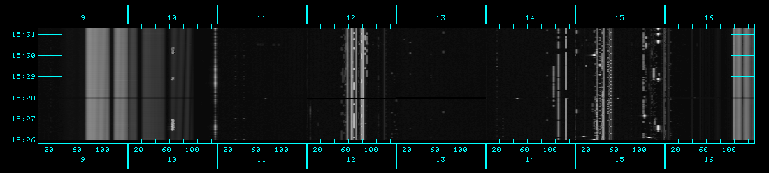 |
| Figure 7.3.1: P-band time vs. frequency for short baseline pair. |
At 4-band, narrow-band RFI is generally not a major issue since most high-power analog TV channels have disappeared with only low-power TV stations transmitting below 100 MHz. Note, the presence of a self-generated RFI comb peaking at 60 MHz with a spacing of 5 MHz at antennas with old antenna control units (ACUs). This issue will improve over time with more antennas having the new generation ACUs. The comb can easily be excised, affecting only a small number of channels. Another hard to detect source of RFI, of particular concern in more compact configurations, is produced by arcing on powerlines. This produces primarily bursts of broad-band noise and can significantly affect the sensitivity of antennas near overhead powerlines and create spurious high cross-correlations. While we try to address powerline issues as they arise, the RFI environment at the VLA is still being evaluated on an ongoing basis.
Solar Activity
While observing at P-band, the following guidelines may be followed while the Sun is quiet:
- In general, make sure that the Sun is more than 30° away from your sources. See the Avoiding the Sun section for more array configuration dependent details.
- In D-configuration, the solar disk will likely cause a problem on the short baselines (< 100m) if the Sun is less than 90° away from the observed source.
- The phases are always calibratable except during solar storms.
When the Sun is active, high solar activity results in emission that can severely affect the data to such a degree as to potentially render your observations useless. Also, such activity causes disturbing ionospheric effects. Therefore, it is imperative to avoid observing at very low frequencies at daytime (including sunrise and sunset†) during times of high solar activity, i.e., when solar flares occur and which are more frequent during solar maximum. Solar flares with as much as a million Jy at P-band with narrow angular extents are a source of major interference. These flares are equivalent to bright, unresolved sources with time-varying flux densities that make it very difficult, if not impossible, to remove their effects. As a consequence, the resulting images will be of poor quality and low dynamic range.
Important Note: It is the responsibility of the observer to monitor if and when their sources will be too close to the Sun in addition to the activity of the Sun. If you do not want your SB(s) executed on the array due to a solar flare, which would take a few days to reach Earth after the occurrence of an eruption on the Sun, you should cancel the submission of your SB(s) through the OPT and resubmit them later. Do not rely on the operator to know about conditions relating to solar flares.
Some useful links:
- Solar activity monitoring: Solar activity and general space weather can be reviewed at the NOAA site. The site provides solar activity forecasts and geophysical (geomagnetic field) activity forecasts along with GOES X-ray flux values.
- Ionosphere monitoring: Global Ionospheric TEC maps or Local Ionospheric Weather from LWA.
- Near real-time and archival solar activity can be seen from < 100 MHz all-sky observations by the LWA.
†Note:The statement to avoid observing at 4/P-band at daytime (including sunrise and sunset) during times of high solar activity should not translate to checking the boxes of AVOID SUNRISE and/or AVOID SUNSET in the OPT, because these will not prohibit observing at daytime during a solar flare event. Also, these options in the OPT are not meant to address or avoid solar activity, but to avoid ionospheric phase fluctuations for low frequency observations and strong temperature gradients for high frequency observations during sunrise and sunset.
Instrument Configuration
There are three different instrument setups available to observe with the VLA at 4 and P-band:
- P-band setup: Provides 16 subbands from the A0/C0 IF pair, each 16 MHz wide, to cover the frequency range 224-480 MHz, with a channel resolution of 125 KHz. The correlator integration time of this setup is 2 seconds with the 8-bit samplers.
- 4-band setup: Provides 8 subbands from the B0/D0 IF pair, each 4 MHz wide, to cover the frequency range 54-86 MHz, with a channel resolution of 15.6 kHz. The correlator integration time of this setup is 2 seconds with the 8-bit samplers.
- 4&P-band setup: This combined the two setups from above to observe 4 and P-band simultaneously.
Requantizer Setup Scans
We strongly recommend using requantizer gain level setup scans in very low frequency observations. Here we note two important sections on the use of these setup scans in 8-bit observations:
- See the 8-bit General Information section under the '8/3-bit Attenuator Settings and Setup Scans' page of the VLA Observing Guide for information on how to trigger the requantizer gain setup scans while using the 8-bit samplers.
- See the Special Case II in the '8/3-bit Attenuator Settings and Setup Scans' page of the VLA Observing Guide for the reasons to use the requintizer setup scans in P-band observations, and the current implementations in the Observation Preparation Tool (OPT) to utilize such scans.
Calibration
A number of calibrator observations are needed for the 4 & P-band observations. These usually include: flux density scale calibrator, complex gain (phase and amplitude gain) calibrator, and a bandpass calibrator to correct for the delays as well as the relative gains of the spectral channels even though the observations are intended for continuum science. It is recommended that the flux density calibrator be observed at least once in an observing run (a scheduling block).
Absolute Flux Density Scale
Accurate flux densities can be obtained by observing one of 3C48, 3C123, 3C138, 3C147, 3C196, 3C286, 3C295, or 3C380. P-band models are available for these sources, or at minimum a subset of, in CASA or AIPS, therefore if a given calibrator is resolved (see the VLA calibrator list), make sure to set appropriate uv ranges while executing calibration tasks. For more details on flux density calibration, see the AIPS task SETJY or the CASA task setjy.
Bandpass (and Delay)
For the VLA it is essential to calibrate the spectral response of each correlator mode used, even for purely continuum projects. For P-band observations it is necessary to use a calibrator that is > 40 Jy to properly calibrate the bandpass response, this includes continuum and spectral line projects. Some of the flux density calibrators noted above can be used for bandpass calibration at P-band. The bandpass calibrator can also be used to calibrate the delays. For calibration of 4-band data it is strictly necessary to observe a bright kJy-scale calibrator to solve for delays and bandpass. The by far single best calibrator is Cygnus A, however if observing at the galactic anticenter, depending on the array configuration and resolved structure, Taurus A or Virgo A might be suitable as well. For more details, refer to the Bandpass and Delay Calibration in the Calibration section, or the Spectral Line section.
Complex Gain (phase and amplitude gain)
Considering the large field of view of very low frequency observations, it will always be possible to self-calibrate the target phases because there will be a strong source or several strong sources within the field. It is recommended, however, to observe a complex gain calibrator (flux density > 10 Jy) with a gain cal + target + gain cal time of 30 to 60 minutes regardless of the array configuration for initial calibration and system monitoring purposes.
For more details on the above calibrators, refer to the Calibration section.
For information on rapid phase calibration and the Atmospheric Phase Interferometer (API), refer to the VLA OSS. More details regarding cycle times may be found under the Calibration Cycles of the Calibration section.
Polarization
Polarimetric observations are available for P-band only under SRO. The details for polarimetric calibration are currently being commissioned. Guidance on observation setup and calibration using AIPS is documented in EVLA Memo #207.
At 4-band due to the nature of the dipole response, the sensitivity and beam-shapes are vastly different between the two polarizations. Thus, only continuum imaging is currently commissioned below 100 MHz. It is available to perform polarimetric observations at 4-band through RSRO proposals.
Before submitting a scheduling block (SB), refer to the Presubmission Checklists:
Please submit any questions to the NRAO Helpdesk.
Commonly Used Observing Modes
Spectral Line
The wide bandwidths of the VLA allow users to observe up to 8GHz of bandwidth at a time. All observations with the VLA are inherently spectral observations, including those intended for continuum science. The VLA's improved sensitivity and wide bandwidths greatly enhance the VLA's functionality for spectral line purposes, enabling simultaneous imaging of multiple spectral lines. The WIDAR correlator is extremely flexible and can act as up to 64 independent correlators with different bandwidths, channel numbers, polarization products, and observing frequencies. The VLA is able to:
- deliver continuous spectral coverage of up to 8GHz;
- access 1GHz or 2GHz chunks in each receiver band (called basebands) and place multiple correlator subbands within them;
- place up to 32, independently tunable subbands within a baseband, up to 64 in total. Each subband can be configured with its own subband bandwidth, number of frequency channels, and polarization products;
- fine-tune each baseband frequency independently according to an object's line-of-sight velocity with respect to the earth at the time of the observation (Doppler Setting); each subband frequency can be set to apply this shift or not.
The detailed capabilities offered for each semester are described in the VLA Observational Status Summary (OSS).
Line Frequencies and Velocity Conventions
Spectral line catalogs available online are useful for selecting targeted line rest frequencies. The recommended catalog for VLA and ALMA observing is Splatalogue which contains molecular line data from sources including the Lovas catalog, the JPL/NASA molecular database, the Cologne Database for Molecular Spectroscopy, as well as radio recombination lines.
Observing Frequency and Velocity Definitions
The sky frequency (ν) at which we must observe a spectral line is derived from the rest frequency of the spectral line (ν0), the line-of-sight velocity of the source (V), and the speed of light (c). The relativistic velocity, or true line-of-sight velocity, is related to the observed and rest frequencies by
\[V = \frac{\nu^2_0-\nu^2}{\nu^2_0+\nu^2}c\]
This equation is a bit cumbersome to use; in astronomy two different approximations are typically used:
- Optical Velocity \[V^{optical} = \frac{\lambda-\lambda_0}{\lambda_0}\,\,c = cz \] (z is the redshift of the source; λ and λ0 are the corresponding observed and rest wavelengths, respectively)
- Radio Velocity \[V^{radio} = \frac{\nu_0-\nu}{\nu_0}\,\,c = \frac{\lambda-\lambda_0}{\lambda}\,\,c \neq V^{optical} \]
The radio and optical velocities are not identical. Particularly,V optical and V radio diverge for large velocities. Optical velocities are commonly used for (Helio/Barycentric) extragalactic observations; (LSR) radio velocities are typical for Galactic observations.
At high redshifts, it is advisable to place the zero point of the velocity frame into the source by redshifting the rest frequency of the line via \[\nu=\frac{\nu_0}{z+1}\]
where the redshifted rest frequency ν can now be used as the nominal rest frequency for the observations. Zero velocity is then defined for that redshift and is therefore intrinsic to the object. This method will appropriately apply the redshift correction to the channel and line widths and the resulting velocities are also relative to the source.
Note that the VLA's natural spectral axis is in frequency. The radio convention will simply be a velocity relabeling to the frequency axis. Using the optical velocity and redshift, however, will introduce a non-linearity between channel widths and labeling, in particular for large velocity values.
Velocity Reference Frames
The Earth rotates, revolves around the Sun, rotates around the Galaxy, moves within the Local Group, and shows motion against the Cosmic Microwave Background. As for the convention above, any source velocity must therefore also always be specified relative to a reference frame.
Various velocity rest frames are used in the literature. The following table lists their name, the motion that is corrected for, and the maximum amplitude of the velocity correction. Each rest frame correction is incremental to the preceding row:
| Rest Frame Name | Rest Frame | Correct for | Max. Amplitude (km/s) |
|---|---|---|---|
| Topocentric | Telescope | Nothing | 0 |
| Geocentric | Earth Center | Earth rotation | 0.5 |
| Earth-Moon Barycentric | Earth+Moon center of mass | Motion around Earth+Moon center of mass | 0.013 |
| Heliocentric | Center of the Sun | Earth orbital motion | 30 |
| Barycentric | Earth+Sun center of mass | Earth+Sun center of mass | 0.012 |
| Local Standard of Rest (LSR) | Center of Mass of local stars | Solar motion relative to nearby stars | 20 |
| Galactocentric | Center of Milky Way | Milky Way Rotation | 230 |
| Local Group Barycentric | Local Group center of mass | Milky Way Motion | 100 |
| Virgocentric | Center of the Local Virgo supercluster | Local Group motion | 300 |
| Cosmic Microwave Background | CMB | Local Supercluster Motion | 600 |
The velocity frame should be chosen based on the science. For most observations, however, one of the following three reference frames is commonly used:
- Topocentric is the reference frame of the observatory (defining the sky frequency of the observations). Visibilities in a measurement set are typically stored in this frame.
- Local Standard of Rest is the native output of images in CASA. Note that there are two varieties of LSR: the kinematic LSR (LSRK) and the dynamic (LSRD) definitions for the kinematic and dynamic centers, respectively. In almost all cases LSRK is being used and the less precise name LSR is usually used synonymously with the more modern LSRK definition. LSR in the PST and in the OPT means LSRK.
- Barycentric is a commonly used frame that has virtually replaced the older Heliocentric standard. Given the small difference between the Barycentric and Heliocentric frames, they are frequently used interchangeably.
Doppler Correction
A telescope naturally operates at a fixed sky frequency (Topocentric velocity frame) which can be adjusted to account for the motion of the Earth. The observed frequency of a spectral line will shift during an observing campaign. Within a day, the rotation of the Earth dominates and the line may shift up to ±0.5km/s, depending on the position of the source on the sky (see the table on Velocity Rest Frames above). Observing campaigns that span a year may have spectral lines that shift by up to ±30km/s due to the Earth's motion around the Sun.
As a rule of thumb, 1 MHz in frequency corresponds roughly to x km/s for the line at a wavelength of x in mm. For example, 1 MHz corresponds to about 7 km/s in velocity at a wavelength of 7 mm, and to roughly 210 km/s at the 21 cm line. Using this rule of thumb, a line may shift by up to ±5 MHz in Q-band and by up to ±0.15 MHz in L-band over the course of a year. This shifting needs to be taken into account when setting up the dynamically scheduled observations. Accounting for the frequency shifting can be handled in different ways:
- use the same fixed sky frequency for all observations, accommodating the line shift (maximum of ±30 km/s) by using a wide enough bandwidth to cover the line at any time in the observing campaign. The data is later regridded in post processing to a common LSRK or BARY velocity frame. The actual sky frequency of a specific spectral line rest frequency can be computed with the Dopset tool for any given time. One may find the LST dates for an observation on the VLA Observing Schedules page.
- calculate the sky frequency at the beginning of an observing block and keep this fixed for the duration of the scheduling block. This is called Doppler Setting (in contrast to Doppler tracking below). The VLA supports Doppler setting. Doppler Setting can be specified for each individual baseband in the OPT, removing the burden to do this for each possible observing run by the observer. The line shift during the observation is then reduced to the rotation of the earth (maximum amplitude ±0.5 km/s). This small shift will be corrected in data processing, i.e., if the length of the observing run justifies this correction. Although the absolute sky frequency will be different between observing runs separated in time, Doppler Setting will place the spectral line in the same channel number of each repeated observation.
- change the sky frequency continuously to keep the line at the same position in the band. This method is called Doppler tracking and was standard for the VLA before the WIDAR correlator was in place. Now, the VLA does NOT support Doppler tracking. The WIDAR correlator offers enough bandwidth and spectral channels to cover any line shift and post processing regridding needs. Additionally, a non-variable sky frequency may also yield a more robust calibration and overall system stability.
The regridding of the spectrum can be completed during data processing in CASA directly during imaging in the tasks clean and tclean. Tasks cvel or mstransform provide the same functionality for the visibilities in a MeasurementSet without imaging. In AIPS, the task CVEL typically is run after bandpass calibration. Assuming one knows the spectral line width in advance, the regridding works well when the spectral features are sampled with at least 4 channels. We therefore recommend to oversample an spectral feature with at least 4 channels during the observations.
The WIDAR Correlator
The WIDAR correlator is inherently a spectral line correlator in any regular mode. A full description of the current WIDAR capabilities is provided in the WIDAR section of the OSS. The OSS also contains a spectral line configurations section.
There are two important issues when configuring the WIDAR correlator for spectral line observations. One is to set the necessary spectral resolution. This can be achieved by baseline board stacking and/or recirculation. Both are described in the OSS. For observing large instantaneous bandwidths with high spectral resolution, it is recommended to use as wide as bandwidth as possible (i.e., 128, 64 or 32 MHz) and use stacking, possibly in combination with recirculation over the alternative of using many narrow subbands stacked next to each other. This avoids the stitching process described below and provides a much better spectral baseline.
A second issue is the existence of the 128 MHz boundaries. Lines should not be placed across or very near these boundaries since subbands cannot span across a boundary and the sensitivity drops near the boundaries. In particular note that the very center of the baseband always falls on a 128 MHz boundary. The spectral line under consideration should never be placed in the very center of a baseband. Multi-line observations also need to ensure that none of the lines fall on or near a boundary. This can be challenging at times but is usually a solvable problem and the OPT provides some tools to do so. If it is not possible to obtain simultaneous coverage of all of your lines, or if the exact position of the line is unknown (e.g., for line searches), it is possible to observe with two basebands shifted by 10–64 MHz apart. This will ensure that one baseband covers the boundaries of the other baseband with full sensitivity. An example is given in the figures (8.1.1 and 8.1.2) below, where the top figure shows the RMS of a single baseband with the 128 MHz boundaries sticking out as having high noise. The bottom figure shows a combination of two basebands that have been separated by 64MHz. The noise spikes are clearly suppressed by adding, with the appropriate weight, the two basebands, or even by simply replacing the noisy channels of each baseband with data from the other.
| Figure 8.1.1: Blank field RMS, single 1GHz baseband. Subband edges at 128MHz show increased noise. |
| Figure 8.1.2: Blank field RMS, same as top, but now a combination of two 1GHz basebands shifted by 64MHz. Subband edges are replaced by channels from subbands of the second, frequency shifted baseband. |
Subband 0
The baseband response is suppressed at each side of the spectrum. The largest affected baseband edge is at the highest sky frequency in the baseband when using lower sideband in X and Ku-bands, and at the lowest sky frequency in the baseband when using upper sideband in observing bands other than X and Ku-bands. For upper sideband, this causes reduced sensitivity typically in the lower 20% frequency edge of the first 128 MHz subband and about 5% in the higher frequency edge of the last 128 MHz subband of a baseband (the reverse is happening for X and Ku-bands). It is typically noticed in subband 0 of a baseband, but other subband numbers are possible as well. This part of the spectrum, the lower ~30 MHz and upper ~8 MHz of each baseband in 4, P, L, S, C, K, Ka, and Q-bands or the lower ~8 MHz and upper ~30 MHz of each baseband in X and Ku-bands, should be avoided for spectral line observing if possible. This effect can readily be seen in the figures 7.1.1 and 7.1.2 above, where the RMS in the subband below 4.6 GHz is significantly increased. See EVLA memo 154 for details.
Data Rate Limits
A high number of subbands, baseline board stacking, recirculation, and time resolution can add up to an extremely high data rate in the correlator. Please see the OSS for the allowable data rates and volumes for each observing semester. The OPT instrument configuration calculates data rates based on the spectral line setup and the sum of data rates and total volume must not exceed the maximum allowed for any observational setup.
Preparing Spectral Line Observations
The Observation Preparation Tool (OPT) is the web-based interface to create scheduling blocks (SBs) for time awarded on the VLA. An SB is the observing schedule used for a single observing run. This consists of at least a start-up scan sequence (see the 8/3-Bit Attenuation and Setup Scans guidelines), a bandpass calibrator, a flux density calibrator, a complex gain calibrator, and target observations. High frequency observations should also include at least two (often more) X band interferometric pointing scans and a corresponding setup scan, whereas 3-bit and multi-frequency band observations add even more required scans to the SB. In the OPT, the observer specifies the sources, scan lengths and order, and correlator setups. A full project may consist of several SBs. To access the OPT, go to my.nrao.edu and click on the Obs Prep tab, followed by Login to the Observation Preparation Tool. Instructions for using the OPT and for selecting appropriate calibrators are provided in the OPT Manual.
Bandpass Setup
All observations with the VLA—even those with the goal of observing continuum—require bandpass calibration. When scheduling the bandpass calibration scans within an SB, the observer should be careful to minimize the number of shadowed antennas, as an antenna without a bandpass determined for it will essentially be flagged in the data for the rest of the observation. A bandpass calibrator should be bright enough, or observed long enough, so that the bandpass calibration does not significantly contribute to the noise in the image. For a given channel width a bandpass calibrator with flux density Scal observed for a time tcal and a science target with flux density Sobj observed for a time tobj,  should be greater than
  . How many times greater will be determined by one's science goals and the practicalities of the observations, but should be greater by at least a factor of two. For extremely narrow channels or very weak bandpass calibrators, those typical flux requirements can lead to extremely large integration times. As an alternative one may then choose to reduce the integration time and interpolate in frequency, or to fit a polynomial across all channels in post-processing (bandtype=BPOLY in CASA's bandpass task).
The bandpass calibrator should be a point source or have a well-known model. At low frequencies, the absolute flux density calibrators (3C48, 3C147, or 3C286) are quite strong and can often double as bandpass calibrators. At high frequencies (Ku, K, Ka, and Q-bands), however, these sources have only moderate flux densities of ~0.5–3 Jy, translating into a potentially noisy bandpass solution. A different, stronger bandpass calibrator should then be observed. Naturally, all of the above depends on the channel widths, and for wide channels the standard flux calibrators may be sufficient even at higher frequencies. In turn, extremely narrow channels may require stronger bandpass calibrators at the low frequency end. Additionally, we have shown that one can transfer the bandpass from a wide subband onto a narrow subband if the wide bandpass frequency range covers the narrow one. This may be good to a level of a few percent, but we advise to use that option only when absolutely necessary.
The stability of bandpasses as a function of time is of concern for high-dynamic-range spectral work as well as for weak broad lines. We have found that most antennas show bandpasses that are stable to a few (~2–4) parts in a thousand over a period of several (~4–8) hours. This should be sufficient for most scientific goals but the bandpasses can be observed several times during an observation for extreme calibration accuracy requirements.
A complication can occur when the frequency range of the bandpass is contaminated by other spectral features, such as RFI lines or Galactic HI in absorption or emission. There are two basic options to accommodate that situation:
- if the feature is narrow, one can simply observe as usual. In post processing, the narrow feature can be flagged and the frequency gap interpolated by values of nearby channels or by fitting a polynomial across the bandpass.
- for wider contaminating lines, an option is to observe the bandpass at slightly offset frequencies and transfer the bandpass to the target frequency. If a common solution is obtained from two, symmetric offsets, at higher and lower frequencies, the solution can be improved. Depending on the choice of offsets, and also on the position in the receiver frequency range, the error can vary. For 4 MHz offsets close to the HI rest frequency of 1.42 GHz, the error is in the percent range.
Complex Gain Calibration
The complex gain (phase and amplitude gain) calibration is the same for a spectral line observation as for any other observation. Ideally, one should use the same correlator setup for the complex gain calibrator and the science target. For weak calibrators, however, it is possible to use wider bandwidths for the phase calibrator and then transfer the phases to the source. However, there will be a phase offset between them. The phase offset between the narrow and wide subbands can be determined by observing a strong source at both setups (e.g. the bandpass calibrator) and applied in post processing from the complex gain calibrator to the target sources. A similar method can be used if the complex gain calibrator is observed at a slightly different frequency, e.g. to avoid a contaminating line feature such as Galactic HI.
Polarimetry
Quick Start Guide
There are two components for polarization calibration:
- Determining the leakage terms (i.e., the polarization impurity between the R and L polarizations).
- Calibrating the absolute polarization angle.
There are two common approaches to determine the leakage terms:
- either observe one or more strong calibrators (> 1 Jy) over a wide range (e.g., > 60 degrees) in parallactic angle and through multiple scans,
- or observe a strong unpolarized (typically less than 1% polarized) calibrator source through at least one scan; see below for more information on determining leakage terms.
To calibrate the absolute polarization angle, observe a calibrator with a well-known polarization angle.
In the following we present detailed information on polarization calibration, including the most common calibrators for this purpose.
Guidelines
For projects requiring imaging in Stokes Q and U, the instrumental polarization can be determined through observations of a bright calibrator source spread over a range in parallactic angle. The phase calibrator chosen for the observations can also double as a polarization calibrator provided it is at a declination where it moves through enough parallactic angle during the observation (roughly Dec 15° to 50° for a few hour track). The minimum condition that will enable accurate polarization calibration from a polarized source (in particular with unknown polarization) is three observations of a bright source spanning at least 60 degrees in parallactic angle (if possible schedule four scans in case one is lost). If a bright unpolarized unresolved source is available (i.e., known to have very low polarization) then a single scan will suffice to determine the leakage terms. The accuracy of polarization calibration is generally better than 0.5% for objects small compared to the antenna beam size. However, to achieve accuracy of polarization calibration to better than a few percent, sufficient signal-to-noise for the leakage calibrator is required to be able to correct for spectral variations in instrumental polarization with typical channel widths of the order of a few MHz. The best results are achieved using an unpolarized calibrator or a bright polarized calibrator with good parallactic angle coverage. More details on different calibration strategies can be found in EVLA Memo #201. At least one observation of 3C286 or 3C138 (or another polarized calibrator with known linear polarization angle) is required to fix the absolute position angle of polarized emission. 3C48 also can be used to fix the position angle at wavelengths of 6 cm or shorter.
High sensitivity linear polarization imaging may be limited by time dependent instrumental polarization, which can add low levels of spurious polarization near features seen in total intensity and can scatter flux throughout the polarization image, potentially limiting the dynamic range. Preliminary investigation of the VLA’s new polarizers indicates that these are extremely stable over the duration of any single observation, strongly suggesting that high quality polarimetry over the full bandwidth will be possible. In addition, geometric effects appear to be limiting the absolute polarization angle calibration especially in cases where a source is observed at opposite sides of transit independent of observing band. A detailed investigation is documented in EVLA Memo #205.
The accuracy of wide field linear polarization imaging will be limited, likely at the level of a few percent at the antenna half-power width, by angular variations in the antenna polarization response. Algorithms to enable removing this angle-dependent polarization are being tested and observations to determine the antenna polarizations have begun. Circular polarization measurements will be limited by the beam squint, due to the offset secondary focus feeds, which separates the RCP and LCP beams by a few percent of the FWHM. The same algorithms noted above to correct for antenna-induced linear polarization can be applied to correct for the circular beam squint. Measurement of the beam squints, and testing of the algorithms, is ongoing.
Ionospheric Faraday rotation of the astronomical signal is always notable at 20 cm. The typical daily maximum rotation measure under quiet solar conditions is 1 or 2 radians/m2, so the ionospherically-induced rotation of the plane of polarization at these bands is not excessive – 5 degrees at 20 cm. However, under active conditions, this rotation can be many times larger, sufficiently large that polarimetry is impossible at 20 cm with correction for this effect. The AIPS program TECOR has been shown to be quite effective in removing large-scale ionospherically induced Faraday Rotation below 2 GHz. It uses currently-available data in IONEX format, which provide a global coarse correction. The effect of this ionospheric Faraday rotation on polarization angles is shown as an example in EVLA Memo #205, in particular see Fig. 3. Please consult the TECOR help file for detailed information. CASA provides a similar capability. With CASA release 4.7 it is possible to correct Faraday rotation effects using the task gencal with caltype='tecim'. The addition of dispersive delay corrections are available experimentally in CASA 5.x releases pending further verification.
Monitoring
The results of a careful monitoring program of these and other polarization calibrators can be found at http://www.vla.nrao.edu/astro/evlapolcal/ for 2011/2012. More recent monitoring data is available from the NRAO archive under project TPOL0003 (typically ran every ~90 days or upon request) for secondary calibrators and under project TCAL0009 (typically ran every ~30 days) for primary linear polarization angle calibrators. There is also a list of calibrator monitoring for VLBA observations starting with the 21A semester. If you would like to request a specific set of sources to be monitored, please submit your request to the VLA Observing department in the NRAO Science Helpdesk.
Observing Recommendations
There are several strategies for deriving the Q/U angle calibration:
- Observation of a primary polarization standard (Category A)
- Observation of a secondary polarization calibrator (Category B with Note 3) with auxiliary monitoring observations to transfer from primary.
This calibration is needed to set the polarization vector angle 0.5*arctan(U/Q) and should be done in all cases.
There are several strategies for deriving the instrumental polarization:
- Single scan observation of a zero polarization source (Category C)
- Several scans (minimum of 3 scans over 60 degrees of parallactic angle) of an unknown polarization source. These can be, but are not limited to sources listed in Category B.
- Two scans of a source of known polarization (Category A or B with transfer)
See Tables 8.2.1-8.2.4 below for Category A-D source catalogs.
Polarization Calibrator Catalog and Selection
The following sources are known to be useable for polarization calibration. These consist of a few "pol standard" sources with known stable polarization (for Q/U angle calibration), plus a number of "bright" sources with "monitored" variable flux densities and polarization. Some of these are seen to have only "moderate variability" and could be used as secondary angle calibrators if you can transfer the angle from the monitoring observations. Assume others (particularly "flat spectrum") are highly variable. There are also a few "bright, low pol" sources available as leakage calibrators (but they can have measurable polarization at high frequencies).
NOTE: Be sure to use the VLA OPT Source catalog to obtain the standard J2000 positions and approximate flux densities.
Calibration Selection Procedure:
- Select Polarization Standard (to calibrate polarization angle Q/U) - optimally select one Category A source and observe at least one scan. The percentage polarization and angle for the known stable calibrators as a function of frequency is tabulated in Table 8.2.6 below. Alternative: use a "moderately variable" Category B calibrator and use monitoring information (available via TPOL0003 in the archive or upon request, see above Monitoring section) to transfer from a primary.
- Select Leakage Calibrator (to determine instrumental polarization) - optimally select one Category C low-polarization source or Category B secondary source in optimal Dec range (see the notes of Tables 8.2.1 and 8.2.2) for PA coverage during run (if long enough). Single scans ok for Category C. Alternative: try a Category D CSO if no other options available.
| Source | Other name | Comments | Notes |
|---|---|---|---|
| J0137+3309 | B0134+329 (3C48) | pol standard (>4GHz) | A1,A2,A3 |
| J0521+1638 | B0518+165 (3C138) | pol standard | A1,A4 |
| J1331+3030 | B1328+307 (3C286) | pol standard | A1,A5 |
Table 8.2.1 Notes:
- A1. Polarized fraction and angle values for these sources is given in Table 7.2.6 below.
- A2. 3C48 is weak at high frequency and somewhat resolved in larger configurations. Depolarized below 4GHz.
- A3. 3C48 has resumed pre-2016 values. For accurate polarization angle calibration, care should be taken that a current model of its polarization properties is available and applied during calibration. This can be obtained from monthly monitoring observations available from the NRAO archive with the project code TCAL0009.
- A4. The flux density scale calibrator 3C138 is currently undergoing a flare. As of January 2025, the change in flux density is greater than 10% at all frequencies greater than 4 GHz (i.e., C-band). At present, the magnitude of the flare is approximately a factor of 2 at K-band, 3 at Ka-band, and 4 at Q-band. Monthly monitoring observations are available for investigators that require an accurate flux density scale when using 3C138. These observations are publicly available in the archive under the project code TCAL0009. A table of scaling factors per band per month from February 2021 onward has been provided.
- A5. 3C286 is our foremost primary calibrator and should be used if available.
| Source | Other name | Comments | Notes |
|---|---|---|---|
| J0359+5057 | B0355+508 (NRAO150) | bright, flat spectrum, monitored upon request, moderate variability | B1 |
| J0555+3948 | B0552+398 | bright, flat spectrum, monitored upon request, moderate variability | B1,B2 |
| J0854+2006 | B0851+202 | bright, flat spectrum, monitored upon request, moderate variability | B1 |
| J0927+3902 | B0923+392 | bright, flat spectrum, monitored upon request, moderate variability | B1,B2 |
| J1310+3220 | B1308+326 | monitored upon request | |
| J2136+0041 | B2134+004 | bright, flat spectrum, monitored upon request, moderate variability | |
| J2202+4216 | B2200+420 (BLLac) | bright, flat spectrum, monitored upon request, moderate variability | B1 |
| J2253+1608 | B2251+158 (3C454.3) | bright, flat spectrum, monitored upon request | B3 |
Table 8.2.2 Notes:
- B1. In optimal Declination range to be used as leakage calibrator with PA coverage. Recommended as calibrators and if necessary can be used as secondary standards with monitoring (TPOL0003).
- B2. Low polarization at low frequencies (L, sometimes S,C), do not use as angle calibrator.
- B3. Highly variable and interesting in its own right.
| Source | Other name | Comments | Notes |
|---|---|---|---|
| J0319+4130 | B0316+413 (3C84) | low pol, bright, flat spectrum, monitored upon request | C1 |
| J0542+4951 | B0538+498 (3C147) | low pol <10GHz, steep spectrum, resolved | C2 |
| J0713+4349 | B0710+439 | low pol, CSO, monitored upon request | C3 |
| J1407+2827 | B1404+286 (OQ208) | low pol, steep spectrum | C4 |
| J2355+4950 | B2352+495 | low pol, CSO, monitored upon request | C3 |
Table 8.2.3 Notes:
- C1. Very bright and low polarization (<1%), but variable flux density. Approaches 1% polarized at 43 GHz.
- C2. Steep spectrum and resolved, low polarization below 10GHz (best <4.5GHz). Stable polarization above. About 6% polarized at 43 GHz See Table 7.2.6 below.
- C3. Weak at high frequency, but stable flux and very low polarization.
- C4. Very weak at high frequency, bright and low polarization below 9GHz.
The following northern sources are known to be CSO (Compact Symmetric Objects) and are characteristically unpolarized. They can be used over a range of frequencies (Gugliucci, N.E. et al. 2007, ApJ 661, 78) as "low pol" leakage calibrators. CSOs tend to be on the weak side and should be used with care at higher frequencies. We have not used these with the VLA and thus rate them as "secondary" unpolarized calibrators. Let us know if you use these so we can evaluate their performance.
| Source | B1950 Name | Comments |
|---|---|---|
| J0029+3456 | 0026+346 | CSO |
| J0111+3906 | 0108+388 | CSO |
| J0410+7656 | 0404+768 | CSO |
| J1035+5628 | 1031+567 | CSO |
| J1148+5924 | 1146+596 | CSO |
| J1400+6210 | 1358+624 | CSO |
| J1815+6127 | 1815+614 | CSO |
| J1823+7938 | 1826+796 | CSO |
| J1944+5448 | 1943+546 | CSO |
| J1945+7055 | 1946+708 | CSO |
| J2022+6136 | 2021+614 | CSO |
Another potential set of unpolarized sources (verified only for S band) below 34 degree declination near 3C 48 and 3C 286 are listed in Table 8.2.5. However, like in the case of sources listed in Table 8.2.4, we strongly encourage to let us know before using these secondary unpolarized calibrators due to potential source variability.
| Source | Minimum Flux Density 2-4 GHz (Jy) |
Polarization Fraction 2-4 GHz (%) |
Comments |
|---|---|---|---|
| J0022+0014 | 1.3 | <=0.03 | AGN? |
| J0318+1628 | 3.4 | <=0.04 | LSP Quasar |
| J0329+2756 | 0.9 | <=0.09 | AGN? |
| J1326+3154 | 2.6 | <=0.07 | Radio Galaxy/CSO |
Final Recommendations:
- at least one "pol standard" (ideally from Category A) should be included for angle calibration
- "bright" sources are easily useable as leakage calibrators with PA coverage (and probably good for bandpasses to boot!)
- "monitored" sources can be found at http://www.vla.nrao.edu/astro/calib/polar/ (for VLA 1999–2009) and http://www.vla.nrao.edu/astro/evlapolcal (for VLA 2010-2012), as well as in the NRAO archive under project code TCAL0009, with regular observations since 2016.
- "steep spectrum" sources are likely weak at high frequencies
- "flat spectrum" sources are likely bright at high frequencies but variable
- "moderately variable" sources may be useable in a pinch if you can get a nearby (in time) monitoring observation
Primary Polarization Calibrator Information
At least one observation of 3C286 or 3C138 is recommended to fix the absolute position angle of polarized emission. 3C48 also can be used for this at frequencies of ~3 GHz and higher, or 3C147 at frequencies above ~10 GHz. Table 8.2.6 shows the measured fractional polarization and intrinsic angle for the linearly polarized emission for these four sources in December 2010. Note that 3C138 and 3C48 are variable—the polarization properties are known to be changing significantly over time, most notably at the higher frequencies. See the "Integrated Polarization Properties of 3C48, 3C138, 3C147, and 3C286" (2013, ApJS 206, 2) by Perley and Butler for more details.
| Freq. | 3C48Pol | 3C48Ang | 3C138Pol | 3C138Ang | 3C147Pol | 3C147Ang | 3C286Pol | 3C286Ang |
|---|---|---|---|---|---|---|---|---|
| GHz | % | Deg. | % | Deg. | % | Deg. | % | Deg. |
| 1.05 | 0.3 | 25 | 5.6 | −14 | <0.05 | — | 8.6 | 33 |
| 1.45 | 0.5 | 140 | 7.5 | −11 | <0.05 | — | 9.5 | 33 |
| 1.64 | 0.7 | −5 | 8.4 | −10 | <0.04 | — | 9.9 | 33 |
| 1.95 | 0.9 | −150 | 9.0 | −10 | <0.04 | — | 10.1 | 33 |
| 2.45 | 1.4 | −120 | 10.4 | −9 | <0.05 | — | 10.5 | 33 |
| 2.95 | 2.0 | −100 | 10.7 | −10 | <0.05 | — | 10.8 | 33 |
| 3.25 | 2.5 | −92 | 10.0 | −10 | <0.05 | — | 10.9 | 33 |
| 3.75 | 3.2 | −84 | — | — | <0.04 | — | 11.1 | 33 |
| 4.50 | 3.8 | −75 | 10.0 | −11 | 0.1 | −100 | 11.3 | 33 |
| 5.00 | 4.2 | −72 | 10.4 | −11 | 0.3 | 0 | 11.4 | 33 |
| 6.50 | 5.2 | −68 | 9.8 | −12 | 0.3 | −65 | 11.6 | 33 |
| 7.25 | 5.2 | −67 | 10.0 | −12 | 0.6 | −39 | 11.7 | 33 |
| 8.10 | 5.3 | −64 | 10.4 | −10 | 0.7 | −24 | 11.9 | 34 |
| 8.80 | 5.4 | −62 | 10.1 | −8 | 0.8 | −11 | 11.9 | 34 |
| 12.8 | 6.0 | −62 | 8.4 | −7 | 2.2 | 43 | 11.9 | 34 |
| 13.7 | 6.1 | −62 | 7.9 | −7 | 2.4 | 48 | 11.9 | 34 |
| 14.6 | 6.4 | −63 | 7.7 | −8 | 2.7 | 53 | 12.1 | 34 |
| 15.5 | 6.4 | −64 | 7.4 | −9 | 2.9 | 59 | 12.2 | 34 |
| 18.1 | 6.9 | −66 | 6.7 | −12 | 3.4 | 67 | 12.5 | 34 |
| 19.0 | 7.1 | −67 | 6.5 | −13 | 3.5 | 68 | 12.5 | 35 |
| 22.4 | 7.7 | −70 | 6.7 | −16 | 3.8 | 75 | 12.6 | 35 |
| 23.3 | 7.8 | −70 | 6.6 | −17 | 3.8 | 76 | 12.6 | 35 |
| 36.5 | 7.4 | −77 | 6.6 | −24 | 4.4 | 85 | 13.1 | 36 |
| 43.5 | 7.5 | −85 | 6.5 | −27 | 5.2 | 86 | 13.2 | 36 |
Since 3C48, 3C138, and 3C147 are variable above 10 GHz, we have performed new observations of these calibrators across the band January 31/February 1st, 2019. The updated values from this observation are listed below.
| Freq. | 3C48Pol | 3C48Ang | 3C138Pol | 3C138Ang | 3C147Pol | 3C147Ang | 3C286Pol | 3C286Ang |
|---|---|---|---|---|---|---|---|---|
| GHz | % | Deg. | % | Deg. | % | Deg. | % | Deg. |
| 1.02 | 0.3 | 4.3 | 5.5 | -13 | <0.05 | — | 8.6 | 33 |
| 1.47 | 0.5 | -34 | 7.8 | -9.6 | <0.05 | — | 9.8 | 33 |
| 1.87 | 0.9 | 23 | 9.0 | -9.3 | <0.04 | — | 10.1 | 33 |
| 2.57 | 1.6 | 67.1 | 9.9 | -10 | <0.04 | — | 10.6 | 33 |
| 3.57 | 2.9 | -84 | 10.3 | −9.5 | <0.05 | — | 11.2 | 33 |
| 4.89 | 4.3 | -72 | 10.5 | -10.5 | 0.16 | -13 | 11.5 | 33 |
| 6.68 | 5.4 | -66 | 10.2 | -11.5 | 0.51 | -57 | 11.9 | 33 |
| 8.43 | 5.4 | -63 | 10.9 | -9.4 | 0.48 | -19 | 12.1 | 33 |
| 11.3 | 5.7 | -62 | 9.1 | -7.9 | 0.85 | 27 | 12.3 | 34 |
| 14.1 | 6.1 | -63 | 8.2 | -11 | 1.8 | 53 | 12.3 | 34 |
| 16.6 | 6.3 | -64 | 8.2 | -13 | 2.4 | 60 | 12.5 | 35 |
| 19.1 | 6.5 | -68 | 8.4 | -16 | 2.9 | 66 | 12.6 | 35 |
| 25.6 | 7.2 | -72 | 8.4 | -18 | 3.4 | 79 | 12.7 | 36 |
| 32.1 | 6.4 | -76 | 8.5 | -19 | 4.0 | 83 | 13.1 | 36 |
| 37.1 | 6.7 | -77 | 8.7 | -20 | 4.5 | 87 | 13.5 | 36 |
| 42.1 | 5.6 | -84 | 8.8 | -23 | 4.9 | 87 | 13.4 | 37 |
| 48.1 | 6.8 | -84 | 9.2 | -24 | 6.0 | 85 | 14.6 | 36 |
Link to Flux Density Scale, Polarization Leakage, and Polarization Angle text files.
Summary of Polarization Calibrator Monitoring
More details and up-to-date information on the regular and ad-hoc VLA polarization calibrator monitoring observations can be found on this confluence page.
Subarrays
The VLA can be split up in subarrays. That is, a subset of the 27 antennas and corresponding baselines can be ordered to do a completely different and independent program than other antennas. This may be the case when an observer has asked to divide up the array for a single project to observe a source simultaneously in multiple bands, to observe multiple different sources simultaneously that do not need the full array, or when one antenna is split off from the main array for inclusion in a VLBI array by another user (i.e., Y1).
The current restrictions for observing with subarrays are:
- The use of subarrays has to be requested in the proposal and approved by the TAC.
- Up to 3 subarrays may be used. Note that the array cannot be divided up in three equal subarrays of nine antennas. The following are the allowed subarray allocations.
| 3-subarrays | 2-subarrays |
| (11, 8, 8) | (15, 12) |
| (12, 8, 7) | (16, 11) |
| (12, 11, 4) | (19, 8) |
| (15, 8, 4) | (20, 7) |
| (16, 7, 4) | (23, 4) |
| (16, 8, 3) | (24, 3) |
| (19, 4, 4) | |
| (20, 4, 3) | |
- For more information see the subarray configuration details in the VLA OSS.
- 8-bit and 3-bit default NRAO wideband continuum frequency setups may be used for standard interferometric observing (no phasing, binning, etc., and no spectral lines). Other modes may be offered as RSRO in the call for proposals.
- The division of observing directions, frequency bands, polarization products and integration times over subarrays is unrestricted. Observations where the correlator configuration changes within a given subarray are currently allowed as SRO. OTF modes are not supported in subarray observations.
- Only a single scheduling block should be submitted through the OPT, with appropriate comments to the operator. This scheduling block should consist of Subarray Loops, one per subarray in which separate lists of scans are placed for each subarray. Each Subarray Loop defines the antennas used per subarray. Check the OPT manual before you start making the subarray schedule by referring to the Subarray Observing section.
- The sum of data rates and other restrictions and guidelines for standard (single subarray) observations must be taken into account.
- All Subarray Loops in a single Scheduling Block are started at the same time.
Please review the Subarray Observing section in the OPT manual for further information or contact the NRAO Helpdesk.
Mosaicking and OTF
This document is intended for observers planning VLA observations using multiple pointing and phase centers to create a "mosaic". A mosaic is an image of a patch of sky that is made up of more than one observed field.
Mosaicking should be used when the desired field of view (patch of sky to be observed) is relatively large compared to the Primary Beam at the highest observing frequency (as defined in the Field of View section of the VLA OSS). Per definition of the Primary Beam (θPB), the image sensitivity will decrease with distance from the center of the field according to a Gaussian with FWHM=θPB. Thus, the sensitivity at a distance θPB from the pointing center will be worse by a factor of two as compared with the pointing center. To achieve approximately constant sensitivity over the field of view, the field of view must be << θPB. If the loss in sensitivity at the edge of the field of view is not acceptable, the observations should be made using a mosaic rather than a single pointing.
Note: The Largest Angular Scale (LAS) that can be imaged by the array is independent of both the Primary Beam and the use of mosaicking to increase the field of view. A table of the band- and configuration-dependent LAS is presented in the Resolution section of the OSS.
Mosaic observing with the VLA
There are two different ways of observing a patch of sky that is much larger than the telescope's instantaneous field-of-view. The standard approach, known as a discrete or pointed mosaic, is to combine together fields from individual pointings of the telescope. This method is typically used for smaller and/or non-rectangular patterns or when significant time needs to be spent per sky area to obtain sufficient sensitivity and image fidelity. The other approach, known as On-The-Fly mapping or OTF(E), combines data that is taken in a 'scanning' mode, where the telescope does not dwell on a position but keeps moving with respect to the sky. OTF is most useful to scan large rectangular patterns on the sky such as for shallow surveys and transient searches where at least one dimension of the mosaic is many times larger than the primary beam. Each method has their advantages, prerequisites, and limitations. Whether to choose one over the other depends on the science goal and boundary conditions such as sensitivity but also, e.g., data rate.
Important considerations are:
- size and shape of the area to cover (in primary beams)
- sensitivity of the observation over the area (amount of integration time required on any single field of the mosaic)
- image requirements (e.g., uv-coverage and largest angular size)
The VLA supports, through General Observing, mosaics that use a discrete pointing pattern. In this standard mode, the mosaic pointing centers are set up as individual fields to be observed (as if they were just a set of target sources). In data post-processing, the data that come from these groups of mosaic fields are jointly deconvolved taking into account the mosaic patterns.
Since semester 2015A, as part of our Shared Risk Observing (SRO) program, the VLA has been offering the opportunity to use OTF mosaicking to more efficiently scan large areas with small dwell times on each point. This is done by moving the telescopes while taking data (and stepping the phase centers for correlation). Special considerations must be taken in processing data taken with this mode. See the section Considerations for On-The-Fly (OTF) Mosaics below and the OPT Manual section on OTF for more details. Observers considering the use of OTF mode are encouraged to contact NRAO staff through the NRAO HelpDesk to ensure the feasibility of their OTF observations.
Preparing for mosaic observing: Discrete or On-The-Fly?
You should only use OTF mosaicking if it will be significantly more efficient than standard mosacking. The great benefit of OTF is the ability to eliminate the settling time (after every antenna move) that is required for each pointing in a discrete mosaic. For the VLA, the settle time typically amounts to 7s per pointing. Therefore OTF is particularly useful for large, shallow mosaics that require <15-25s per mosaic beam, where the settle time per field would amount to a very large overhead (>30%-50%) on the observations.
To determine if the standard approach will work for your purposes, first determine the "required integration time per discrete pointing" using the steps outlined below. If the integration time is >25 seconds, then you should use a standard discrete mosaic. For integration times ranging from 14 seconds to 24 seconds it is a gray area - OTF mosaicking would require less overhead, but the extra processing cost and added complexity probably mean you should use standard mosaicking unless you are familiar with processing this type of data in CASA. However, if your integration time is shorter than about 14 seconds, then the time it will take to move and settle between pointings will incur >50% overhead. Unless this extra overhead is not a problem (i.e. the overall mosaic is quite small in area) you should consider using OTF.
Use the following steps to determine the individual integration times (tinteg) that would be required for discrete pointings. You should go through the following steps to prepare your observations, even if you already know which type of mosaic (discrete or OTF) you plan to observe.
- What area of sky do you want to cover?
- Compute the total mosaic area \(A_{\rm mos}\) in appropriate solid angle units, e.g. square degrees.
- Example
- I want to cover 5 degrees x 5 degrees, so my area is 25 square degrees.
- Compute the total mosaic area \(A_{\rm mos}\) in appropriate solid angle units, e.g. square degrees.
- What is the effective primary beam size in your observing band? How many independent "beams" are in the mosaic?
- Compute the Full-Width Half-Maximum (FWHM) \(\theta_p\) of the VLA at a representative frequency \(v_{\rm obs}\), usually the center of your observing band, using the formula
- \[\theta_P \approx 42^\prime \frac{\rm 1 \: GHz}{\nu_{\rm obs}}\] (see the Field of View section in the VLA OSS document)
- Example
- I am observing in L-band 1-2 GHz, so νobs = 1.5GHz and θP \(\approx\) 28'.
(Note that the formula given above for \(\theta_P\) is approximate, as the beam is not perfectly linear with frequency. For more accurate beam sizes as a function of frequency, we refer the user to EVLA Memo 195 by R. Perley (2016) for the Karl G. Jansky VLA. For beam sizes for the original VLA, we refer the user to VLA Test Memo 134 by Napier & Rots (1982). )
- Compute the mosaic beam area ΩB from the FWHM using the formula \[\Omega_B = 0.5665~\theta^2_P\] (see the Gaussian Beam Pattern Sensitivity subsection below for more details)
- Example
- For my θP = 28' = 0.47° the equivalent mosaic beam area is ΩB = 0.123 square degrees.
- Compute the number of independent/effective beam areas in the mosaic using the formula
- \[N_{\rm eff}=\frac{A_{\rm mos}}{\Omega_B}\]
- Example
- For my 25 square degree mosaic with ΩB = 0.123 square degrees I have 203 effective beams.
- Compute the Full-Width Half-Maximum (FWHM) \(\theta_p\) of the VLA at a representative frequency \(v_{\rm obs}\), usually the center of your observing band, using the formula
- How much integration time do I need? What is my Survey Speed (SS)?
- Compute the integration time per "beam" teff using the VLA Exposure calculator. (Note that teff is the effective integration time for any part of the mosaic, which is not the same as the actual integration time per discrete pointing.)
- Example
- I wish to reach RMS 0.05 mJy. For 600 MHz usable bandwidth at 1.5 GHz in B-configuration with robust weighting and dual polarization, I need 2m47s on-sky.
- Compute the total integration time ttotal for the mosaic by multiplying by the number of beams. (Note: to first order, this is independent of how you actually split up the mosaic.)
- Example
- For 2m47s per beam and 203 beams I need 9h25m total over the mosaic.
- Compute the Survey Speed (SS) by taking the mosaic area and dividing by the total integration time (SS = Amos/ ttotal). This is equivalent to simply computing directly SS = ΩB / teff also!
- Example
- For ttotal=9h25m (9.4 hours) total over the 25 square-degree mosaic, the implied survey speed is about 2.65 square degrees per hour (or equivalently SS = 2.65 square arc-minutes per second).
- Compute the integration time per "beam" teff using the VLA Exposure calculator. (Note that teff is the effective integration time for any part of the mosaic, which is not the same as the actual integration time per discrete pointing.)
- What mosaicking pattern would you wish to employ? What will be the spacing between pointings?
- For discrete/pointed mosaics, we recommend to use a hexagonal mosaicking pattern with a spacing of θhex along rows and θrow ≈ √3 θhex/2 between rows. Typically a value of θhex = θP/√2 is sufficient, but consider using θhex = θP/√3 if uniformity is a strong concern. You might choose to use θP computed from the upper frequency limit of the band, as the highest frequency corresponds to the smallest primary beam (thus the highest frequency will have the lowest uniformity in coverage).
- Example
- For our θP = 28' at 1.5 GHz we get θhex = 19.8' for the spacing along rows and θrow = 17'9" (1029") between rows. This will be more under-sampled at the upper band edge of 2GHz, and over-sampled at 1GHz, but for our basic observations this should be OK.
- For discrete/pointed mosaics, we recommend to use a hexagonal mosaicking pattern with a spacing of θhex along rows and θrow ≈ √3 θhex/2 between rows. Typically a value of θhex = θP/√2 is sufficient, but consider using θhex = θP/√3 if uniformity is a strong concern. You might choose to use θP computed from the upper frequency limit of the band, as the highest frequency corresponds to the smallest primary beam (thus the highest frequency will have the lowest uniformity in coverage).
- How many discrete pointings will be required to cover this mosaic?
- To fill a rectangular area, long and short rows should alternate, with 1 extra pointing in the long rows.
- Example
- Our square mosaic has sides of 5 deg (300'). The spacing between rows is θrow = 17'9" (1029") so there should be 17.5 spacings, and we will therefore schedule 18 rows. Our 300'-length rows will have spacing between pointings of θhex = 19.8', so we will observe 16 pointings in the short rows. The beginning and end pointings in each of these short rows will be 15 x 19.8' = 297' apart. The short rows will alternate with longer rows of 17 pointings (16 x 19.8' = 316'8" between the pointings at either end of a long row). We will have 9 short rows interspersed with 9 long rows, or 9 x 16 + 9 x 17 = 297 pointings in our mosaic.
- To fill a rectangular area, long and short rows should alternate, with 1 extra pointing in the long rows.
- How much integration time should be allocated per discrete pointing?
- Divide the total mosaic integration time by the number of mosaic pointings.
- Example
- Our total integration time of 9h25m is spread among 297 pointings, so each pointing should get 1m54s of integration time.
- You may wish to consider using On-The-Fly (OTF) mosaicking if your integration time per pointing is less than 24 seconds; definitely consider it if your integration time is less than 15 seconds.
- Divide the total mosaic integration time by the number of mosaic pointings.
If at this point you think you should use OTF mosaicking, see the section below on Considerations for On-The-Fly (OTF) Mosaics. Or, continue with the following steps to determine the total amount of observing time required (including overhead) for a discrete mosaic.
- Calculate approximate duration (excluding calibration) for the mosaic.
- The VLA slew and settling time for short distance (sub-degree) moves is 7-8 seconds.
- Example
- For 1m54s integrations we add 8s so we can have observations of 2m02s. The total time for 297 pointings is 10h4m.
- The VLA slew and settling time for short distance (sub-degree) moves is 7-8 seconds.
- Calculate schedule overheads.
- Follow the Exposure and Overhead guidelines in the Guide to Proposing for the VLA.
- Example
- For ease of scheduling, we will break our ~10h mosaic into three parts, each with 3h22m of observing time. Our overheads will include: 10m allowance to get on-source at the beginning of each scheduling block, a 10m scan of a flux calibrator, and 3m after every 20m of mosaic observing (10 visits) to observe our gain calibrator. The total time for each scheduling block comes to 4h12m. This amounts to a 25% overhead, which is about average for VLA's low frequencies.
- Follow the Exposure and Overhead guidelines in the Guide to Proposing for the VLA.
- If project is approved, when it comes time to observe, make a schedule or schedules in the OPT.
- We are working on providing some Python tools (e.g. for CASA) that will help set up mosaic observations. Stay tuned. In the meantime, you may wish to externally generate lists of sources and scans that can be uploaded into the OPT, in order to generate all pointings at once. See the Text Files section of the OPT Manual for instructions.
Considerations for On-The-Fly (OTF) Mosaics
The use of OTF mosaicking with the VLA is the subject of ongoing development and commissioning, and as such is only available under the SRO program.
If you decide to use OTF mosaicking, after full consideration of the overheads for discrete pointings, the next question is "Can I use OTF mosaicking for my observations?". The decision depends on the implied scan speeds and dump rates (and thus data rates). Limitations on the allowed correlator dump times tinteg are not just from the allowed data rates (60 MB/s for standard and shared risk observing); there are also physical limitations on how fast the data from the correlator can be handled by the back-end processing cluster. For the current restrictions on integration times, see the OSS section on Time Resolution and Data Rates. Because some use of OTF is still classified as shared-risk (as of 2020B), the data rate limit is nominally 60 MB/s. This means that you can use shorter integration times when choosing OTF as a shared-risk observer, but for efficiency you should not use a shorter integration time than you truly need.
To set up the parameters of the mosaic (e.g. for the purposes of a proposal), start by following the first several steps outlined above. But instead of computing the number of discrete pointings, you will break the OTF mosaic into a number of "rows"; the antennas will slew back and forth one row at a time at a non-sidereal scan rate (R). Use the following steps to determine the row spacing (θrow; similar to the discrete mosaic case), the required scan rate (R) to meet your sensitivity requirement, the integration/dump times (tinteg), and the associated data rates. Effective integration time (teff) and total mosaic time are calculated as before.
The following steps correspond to an example that is appropriate for OTF observing. Suppose you wish to observe 5x10 square degrees in S-band (2-4 GHz) in the B-configuration to a depth of 0.15 mJy. The effective integration time (teff) to reach this sensitivity (robust weighting, dual pol with 1.5 GHz of bandwidth) is 5.35 seconds.
- What is the mosaic beam area? What is my Survey Speed (SS)?
- To determine the Survey Speed (SS = ΩB / teff), we recommend using θP at the middle of the band, so that the sensitivity can be easily related to the band average of a source with a modest non-zero spectral index. (See Steps 2 and 3 from above.)
- Example
- At 3 GHz, the primary beam size is θP =14'. The equivalent mosaic beam area is ΩB = 0.031 square degrees. Therefore the survey speed is 20.75 square degrees per hour, equivalent to 20.75 square arc-minutes per second.
- For OTF mosaics, we recommend θrow = θP/√2 (equal to the spacing of θhex for discrete mosaics above). We recommend using θP computed from the upper frequency limit of the band, as the highest frequency corresponds to the smallest primary beam (thus the highest frequency will have the lowest uniformity in coverage). Because spacings along OTF rows are necessarily small to avoid beam smearing (< 0.1 θP), smaller spacings between OTF rows maintain better homogeneity overall.
- Example
- At 4 GHz, the primary beam size is θP =10.5'. Therefore I will use a spacing between rows of θrow = 7.4'.
- The scan rate R is calculated as \[R=\frac{\rm SS}{\theta_{\rm row}}\]
- Example
- For a survey speed of SS = 20.75 square arcminutes per second and θrow = 7.4 arcmin, I need an OTF scan rate of R = 2.8 arcminutes per second.
- Note that scans from east to west move with the sidereal motion while scans from west to east are counter-sidereal. Therefore, for the same on-the-sky angular scan rate, the east-to-west scans will require faster telescope motion. We do not recommend requesting scan rates faster than about 3 arcmin/sec, even under Shared Risk Observing. As always, you should avoid observing near the Zenith where the azimuthal rate becomes very high.
- With OTF, fast integrations are required so as not to smear the beam while scanning across the sky. We recommend to have at least 10 samples (integrations) as the antennas scan a distance equal to the FWHM of the primary beam. Therefore the integration time should comply with the formula \[t_{\rm integ}<0.1\frac{\theta_P}{R}\]
- Example
- For the primary beam FWHM at 4 GHz (θP =10.5') and a scan rate of R=2.8'/s, the maximum tinteg to avoid beam smearing is 0.5 seconds.
- Use the OSS section on Time Resolution and Data Rates to determine the data rate.
- Example
- I will base my correlator tuning on the standard setup S-band for B-configuration, using 16 subbands of 128 channels each in dual polarization. For an integration time of tinteg=0.5s, this yields a data rate of 22.5 MB/s which is within the standard observing limit of 60 MB/s.
- Currently we do not allow phasecenter changes in OTF mode faster than 0.6 seconds. Furthermore, we recommend keeping the phasecenter constant for at least 1s for 8-bit modes with 16 sub-bands, and for at least 4s for more than 16 sub-bands per polarization (e.g., with 3-bit continuum modes). If integration times faster than these phasecenter changes are needed, you can request multiple integrations per phasecenter in the OPT.
- Example
- I want to use a dump time of 0.5s, so I will request two integrations per phasecenter. This means the phasecenter will change once per second.
- Determine the amount of time and number of phasecenters to complete one row. An additional preparatory step, with the timing of one additional phasecenter, will be added at the beginning of each row to allow the array to accelerate from rest. The acceleration occurs from a starting position such that the antennas are at the appropriate velocity at the true start position of the OTF row. Make sure to account for the slew-and-settle time between rows, which adds about 10s per row.
- Example
- The phasecenter will change on a cadence of 1 second, and the scan rate R is 2.8 arcmin/sec. Therefore every phasecenter will correspond to 2.8 arcmin of distance scanned. To scan a length of 10 degrees = 600 arcmin across the mosaic in one direction requires N=215 phasecenters. Including the starting acceleration, the scan duration will be (N+1) * 1s = 3m36s per OTF row. Adding in 10s for slew-and-settle time, this comes out to 3m46s per row.
- Note: We currently advocate OTF mosaics where the stripes are at constant Declination. You will want to switch directions for each row so as to scan back and forth (e.g., from west to east for one row, then from east to west for the next, etc.). For mosaics that are very large in the RA direction, you may wish to split the mosaic into several sections so that an individual row is not too long - scanning a long distance in RA can make it difficult to keep your observations above a reasonable elevation limit while maintaining the flexibility of dynamic scheduling. For example, a mosaic with an RA range of 0h to 3h might be broken into three sections (0-1h, 1-2h, 2-3h), with all of the different declination stripes for one RA range observed as a group before moving to the next section.
- Determine the total number of OTF rows to cover the mosaic, and the total time to cover the mosaic.
- Example
- With each row separated by 7.4 arcmin, I will need 41 rows to cover the 5-degree height of the mosaic. The full OTF mosaic will therefore require about 2h35m to observe.
- Follow the Exposure and Overhead guidelines in the Guide to Proposing for the VLA.
- Example
- Our overheads will include: 10m allowance to get on-source at the beginning of each scheduling block, a 10m scan of a flux calibrator, and 3m after about every 4 rows (15m) of OTF observing (11 visits total) to observe our gain calibrator. The total time comes out to 3h28.
- You will need to generate a source list that contains both the starting and ending position of each individual OTF row. You may wish to externally generate lists of sources and scans that can be uploaded into the OPT. See the Text Files section of the OPT Manual for instructions on setting up OTF observing schedules.
Survey Speed of the VLA for Large Continuum Mosaicked Surveys
Following the above guidelines, we can compute the survey speed SS \[SS = \Omega_B / t_{eff} = 0.5665~\theta^2_{P} / t_{eff}\] of the VLA for our standard bands calculated at a given depth in RMS image sensitivity. We choose a "RMS Noise" of 0.1 mJy/beam in the Exposure Calculator (also 25 antennas, natural weighting, dual polarization, medium elevation, autumn weather, B-configuration) to compute the effective integration time, teff. From this, we calculate SS from θP at band center.
The parameters are tabulated by band below:
| Band (freq) | Freq. | Bandwidth | teff (sec) | θP (arcmin) | SS (deg2/hr) |
|---|---|---|---|---|---|
| P (230-470MHz) | 370 MHz | 200 MHz | 5940 | 135' | 1.74 |
| L (1-2GHz) | 1.5 GHz | 600 MHz | 29 | 28' | 15.32 |
| S (2-4GHz) | 3 GHz | 1500 MHz | 8.3 | 14' | 13.38 |
| C (4-8GHz) | 6 GHz | 3.03 GHz | 4.4 | 7' | 6.31 |
| X (8-12GHz) | 10 GHz | 3.50 GHz | 2.9 | 4.2' | 3.45 |
| KU (12-18GHz) | 15 GHz | 5.25 GHz | 3.5 | 2.8' | 1.27 |
| K (18-26.5GHz) | 22 GHz | 7.20 GHz | 6.9 | 1.91' | 0.30 |
| KA (26.5-40GHz) | 33 GHz | 7.20 GHz | 11 | 1.27' | 0.083 |
| Q (40-50GHz) | 45 GHz | 7.20 GHz | 50 | 0.93' | 0.0098 |
For C-band and higher frequencies 3-bit observing is assumed. Representative frequency, integration time, beam width, and survey speed are at approximately mid-band. You can adjust these values for different assumed sensitivity levels and bandwidths (e.g. for line sensitivity) by scaling according to the values that come out of the Exposure Calculator (e.g. SS will scale as the inverse of the integration time). These values are computed in the limit of OTF (continuous) sampling, but should be approximately valid for optimally sampled Hex mosaics also (see below). The beam widths here are approximate (see EVLA Memo 195 by R. Perley, 2016) and are narrow-band. For a wide-band mosaic, see the section below on Effective Primary Beam for a Wideband Mosaic.
The Details: Mosaic Sensitivity
Following are some in-depth calculations of the discrete mosaic sensitivity, provided for users who wants to know the gory details of how the values are calculated. These formulas are generally applicable to mosaics made with any interferometer (e.g. ALMA, ATCA), although some allowances would need to be made in the calculations to allow for non-homogeneous array elements (e.g. with antennas of different sizes as in ALMA+ACA, CARMA).
Gaussian Beam Pattern Sensitivity
We will be assuming a Gaussian pattern \(\theta_g\) for the main beam response (the so-called primary beam pattern) assuming an array of homogeneous antennas. The sensitivity pattern or response to point sources at a distance θ from the pointing center on-sky is given by
\[f(\theta) = e^{-{\frac{\theta^2}{2\theta^2_g}}}\]
The 2-D integral under this function gives the effective Gaussian beam area (solid angle)
\[\Omega_g = 2\pi\theta^2_g\]
For purposes of mosaic coverage, the area under the primary beam squared is relevant (\(f(\theta)^2\)):
\[f(\theta)^2 = e^{-2{\frac{\theta^2}{2\theta^2_g}}} = e^{-\frac{\theta^2}{2(\theta_g/\sqrt{2})^2}}\]
So the effective Gaussian primary beam for a mosaic is equivalent to a Gaussian with half the area:
\[\Omega_B = 2\pi(\frac{\theta_g}{\sqrt 2})^2 = \pi\theta^2_g = \frac{\Omega_g}{2}\]
It is common practice to specify the Gaussian width by the "full-width half-maximum" (FWHM) θP, where
\[\theta_P = \sqrt{(8 \ln 2)}\; \theta_g = 2.3548~\theta_g\]
or
\[\theta_g = 0.4247~\theta_P\]
We can reformulate the response function in terms of the FWHM via substitution:
\[f(\theta) = e^{-\frac{\theta^2}{2\theta_g^2}} = e^{-4 \ln 2 (\frac{\theta}{\theta_P})^2} = 2^{-4 (\frac{\theta}{\theta_P})^2}\]
Our beam areas are
\[\Omega_g = 2\pi\left(\frac{\theta_P}{\sqrt{8 \ln 2}}\right)^2 = 1.1331~\theta^2_P\]
and for the beam-squared
\[\Omega_B = \frac{\pi}{8\ln 2} \theta^2_P = 0.5665~\theta^2_P\]
Effective Primary Beam for a Wideband Mosaic
The above formulas for the Primary Beam are approximations that apply exactly in the case of a narrow-band mosaic. For a wideband (multi-frequency synthesis) mosaic, the effective primary beam depends on the frequency variation of the narrow-band beam widths and the sensitivity as a function of frequency.
The mosaic imaging process weights the data explicitly by assigned weights (e.g., by the rms noise) and implicitly by the beam area at each frequency (because the effective integration time at each frequency is proportional to the beam area). This effect was pointed out by Condon (2015; reference 5) and can be simply calculated as the frequency-weighted mean beam area over the frequency channels \(k\) according to the formula
\[\bar{\Omega}_B = \frac{\Sigma_k\; w_k\; \Omega_{Bk}}{\Sigma_k\; w_k}\]
For uniform weights \(w_k\) = const. and uniform frequency coverage over the band, we can approximate this sum by the integral
\[\bar{\Omega}_B = \frac{1}{\nu_{\rm max} - \nu_{\rm min}}\; \int^{\nu_{\rm max}}_{\nu_{\rm min}}\; d\nu\; \Omega_B(\nu)\]
If we assume the primary beam FWHM scales inversely by frequency, then
\[\bar{\Omega}_B = \frac{\nu_0^2}{\nu_{\rm min}\; \nu_{\rm max}}\; \Omega_B(\nu_0)\]
\[\Omega_B(\nu) = \Omega_B(\nu_0)\; \left(\frac{\nu_0}{\nu}\right)^2\]
or equivalently \(\bar{\Omega}_B = \Omega_B(\bar{\nu})\) where \(\bar{\nu} = \sqrt{\nu_{\rm min}\; \nu_{\rm max}}\) is the geometric mean frequency.
Weighted Image Sensitivity
A mosaic image can be considered to be a weighted sum of individual field image data (\(d_k\)) corrected for the beam response (\(f\)) at each individual pointing:
\[F = \frac{1}{Z}\sum_{k} w(\theta_k) f^{-1}(\theta_k)\; d_k\]
\[Z = \sum_{k} w (\theta_k)\]
where the \(\theta_k\) are the distances to the pointing centers for the image data points dk, \(w(\theta_k)\) is the weight for data point dk, and \(Z\) is the sum-of-weights function. If the image data have equal RMS sensitivity levels σk = σ0 then the optimal weighting gives
\[w(\theta_k)=f^2(\theta_k)\]
and
\[F = \frac{1}{Z}\sum_{k}f(\theta_k)\; d_k\]
\[Z = \sum_{k} f^2 (\theta_k)\]
This image will have the lowest possible RMS noise level, with the variance of \(F\) given by
\[\sigma_F^2 = \frac{1}{Z^2}\sum_k f^2(\theta_k)\sigma_0^2 = Z^{-1}\sigma_0^2\]
which just scales inversely with the sum-of-weights function Z. Since the equivalent integration time at a given point in the mosaic is inversely proportional to the variance (with all other things being equal) then this is given by Z:
\[t_{eff} = Z t_0\]
where t is the integration time per field (assuming a uniformly observed mosaic).
Discrete Mosaic Spacing Considerations
For discrete (as opposed to OTF) mosaicking, the sampling pattern and spacing of pointing centers determines the sensitivity response of the mosaic. The concept of stepping or scanning an interferometer over an area of sky to synthesize a larger image has been around for a long time, see Ekers & Rots 1979 (reference 1) for the conceptual framework.
The simplest pattern is a rectangular mosaic, with pointing centers at vertices of squares. From the perspective that the FFT of the mosaic pattern is a "synthesized beam" in uv-space that sub-samples the antenna voltage patterns, the Nyquist sampling theorem suggests that a spacing of \(\theta_{\rm rect} = \theta_P/2\) or better is needed (e.g. Cornwell 1998, reference 2). This is the spacing of samples on the sky needed to reconstruct the low spatial frequencies on the scale of the primary beam θP. However, if the goal is merely to cover large areas of sky to survey for relatively compact sources, then the spacing limit given by Nyquist sampling of the primary beam can be loosened and wider separations can be used, as long as the dimples in the sensitivity pattern are not too deep for purposes of having a nearly uniform survey over a large area.
The hexagonal-packed mosaic is the classic mosaic observing pattern. It has long been used at the VLA (e.g. for the NVSS, see reference 3) and at the ATCA (see reference 4). This pattern is like a regular rectangular raster but with alternate rows offset by 1/2 field separation, allowing rows to be placed further apart while still getting nearly uniform sensitivity. The mosaic is thus filled by equilateral triangles, with the triangle vertices defining the pointing centers of the pattern.
The ATCA recommended value for \(\theta_{\rm hex} = {\theta_P}/{\sqrt 3}\) is based on Nyquist arguments (see reference 4). For the NVSS survey (reference 3), the authors argued that a spacing not much wider than \(\theta_{\rm hex} = {\theta_P}/{\sqrt 2}\) would be acceptable from a sensitivity perspective, and in fact used a spacing of approximately \({\theta_P}/{1.2}\). This is sufficient (see below) to have a reasonably uniform sensitivity pattern.
For the current VLA, where we have 2:1 bandwidths possible in a given band (e.g. 1-2 GHz, 2-4 GHz), you have to consider the spacing with respect to the primary beam FWHM over the range of frequencies you are going to map together. For example, for observations from 1-2 GHz, setting a spacing of 0.71 FWHM at 1.5 GHz would give a spacing of only 0.94 FWHM at 2 GHz which gives a minimum weight of Zhexmin = 0.586 (see below), but also with significant oversampling of 0.47 FWHM at 1 GHz. You may wish to err on the side of caution in these cases if having more variable sensitivity at the upper band edge is expected to be an issue for you. Note that we have not quantified any imaging consequences from this (e.g. for spectral index maps) so for now these are just some general guidelines.
Recommendation: For most cases where structure on large angular scales is not being imaged, a hex-pattern mosaic with relatively loose spacing of 0.70 - 0.85 FWHM is probably sufficient. If good imaging of large-scale low surface brightness emission is the goal, then a mosaic sampled at the Nyquist spacings or better should be used. In most cases, you can reasonably get away with setting the spacing by the FWHM at the center of your observing band, leaving the mosaic at the upper end of the band less well-sampled while the mosaic at the lower band edge will be better sampled. If for some reason you require excellent sampling over the whole band, then set the spacing using the FWHM at the highest frequency to be safe.
Example: Discrete Hexagonal Mosaic
Each mosaic pointing center has 6 nearest neighbors (hence the hexagonal pattern), with a distance to each given by θhex. For a pixel at a pointing center, counting that point and the 6 neighboring centers, the sum-of-weights is given by
\[Z_{\rm hexmax} = 1 + 6f^2(\theta_{\rm hex})\]
The worst response is at the center of one of the equilateral triangle tiles. The nearest 3 vertices are at distances given by \(\theta_{\rm hex}/{\sqrt 3}\) giving
\[Z_{\rm hexmin} = 3 f^2 (\frac{\theta_{\rm hex}}{\sqrt 3})\]
If NVSS-style image-plane mosaicking is used, then next sets of vertices out will likely not be included in the image due to an imposed cutoff (see reference 3). Assuming a moderately liberal spacing of \(\theta_{\rm hex} = \theta_P/{\sqrt{2}}\) we get:
\[\theta_{\rm hex} = \frac{\theta_P}{\sqrt 2}\]
\[f(\theta_{\rm hex}) = 0.25\]
\[f(\theta_{\rm hex}/\sqrt 3) = 0.63\]
and
\[Z_{\rm hexmax} = 1.375\; \; \; \; \; \; \; \;Z_{\rm hexmin} = 1.191\]
Thus the lowest points in the mosaic weighting pattern are at 0.87 of the maximum (for the NVSS choice, they are at 0.81 of the maximum). Note that the locations at the pointing centers get an equivalent integration time of 1.375 times the individual pointing integrations.
A large hexagonal mosaic of N x M rows and columns will cover a total area of approximately
\[A_{\rm hex} = N \times \theta_{\rm hex} \times M \times \frac{\sqrt 3}{2}\theta_{\rm hex} = \frac{\sqrt{3}}{2} N_{\rm pt}\theta^2_{\rm hex}\]
For a sampling of \(\theta_{\rm hex}= \theta_P/\sqrt{2}\) we get
\[A_{\rm hex} = \frac{\sqrt3}{4}N_{\rm pt}\theta^2_P = 0.7644 N_{\rm pt}\Omega_B\]
for the area under the squared beam defined above. If we observe the mosaic for a total time T with each of the Npt pointings getting the same integration time tint
\[t_{int} = \frac{T}{N_{\rm pt}}\]
then
\[A_{\rm hex}t_{\rm int} = 0.7644 T \Omega_B\]
or using the effective integration time per point in the mosaic
\[A_{\rm hex}t_{\rm eff} = 0.7644 Z\;T \Omega_B\]
For our hexagonal mosaic, the minimum weight is Zhexmin = 1.191 so
\[A_{\rm hex} t_{\rm hexmin} = 0.91 T \Omega_B\]
For practical purposes, as we will see later on, mosaics in general follow the relation that
\[A_{\rm mos} t_{\rm eff} \approx T \Omega_B\]
which can be used to compute the effective integration time on-sky to put into the exposure calculator for RMS sensitivity.
Recommendation: For most cases where you are using a hexagonal (or rectangular or OTF) mosaic with close to the optimal sampling and want the average sensitivity (not the max or min specifically), you can simply use the following to calculate the total integration time needed
\[T \approx t_{\rm eff}\frac{A_{\rm mos}}{\Omega_B}\]
after getting teff from the VLA Exposure Calculator for your needed sensitivity and chosen bandwidth etc.
Example: Discrete Rectangular Mosaic
The use of rectangular mosaics has been deprecated in favor of hexagonal packed mosaics, but there are cases where they are expedient to set up, and they provide an illustrative case leading in to the discussion of on-the-fly mosaics.
For the rectangular mosaic each point is surrounded by eight immediate neighbors with the 4 nearest separated by θrect in the cardinal directions and next 4 by \(\sqrt{2}\theta_{\rm rect}\) on the diagonals. Thus,
\[Z_{\rm rectmax} = 1 + 4 f^2(\theta_{\rm rect}) + 4 f^2(\sqrt{2}\theta_{\rm rect}) = 2.25\]
for the optimal θrect = 0.5 θP.The weight minima have 4 nearest neighbors at θrect/√2
\[Z_{\rm rectmin} = 4 f^2(\frac{\theta_{\rm rect}}{\sqrt 2}) = 2\]
Thus our rectangular mosaic has dimples at 0.89 of the maximum response. The maximum effective integration time is 2.25 times the per pointing integration time. Our mosaic of N rows by M columns covers an area of approximately
\[A_{\rm rect} = N \times \theta_{\rm rec} \times M \times \theta_{\rm rect} = N_{\rm pt}\theta^2_{\rm rect}\]
so going through the same calculation as for the hexagonal mosaic
\[A_{\rm rect} = \frac{1}{4}N_{\rm pt}\theta^2_{P} = 0.4413 N_{\rm pt}\Omega_B\]
and
\[A_{\rm rect}t_{\rm eff} = 0.4413\; Z\; T\; \Omega_B\]
For our rectangular mosaic, the minimum weight is Zrectmin = 2 so
\[A_{\rm rect}t_{\rm rectmin} = 0.88 T \Omega_B\]
The Continuum Limit and On-the-Fly Mosaic Sensitivity
The following are some in-depth calculations of the OTF mosaic sensitivity.
We first calculate the sensitivity in the continuum limit, where the array scans the sky over a given area A in a time T in as uniform a manner as possible. In this case, except near the edges, each point along the row has the same weight, and our sums in the previous derivations become integrals. The image at a given position on the sky (\({\rm\bf x}_0\)) amounts to a weighted integration of the field data (\(D(x)\)) over all nearby sky positions (\({\rm\bf x}\)) corrected by the beam response (\(f\)), and keeping in mind that the beam scans across the sky over time:
\[F({\rm x_0}) = \frac{1}{Z}\int dt\; w({\rm\bf x-x_0})\; f^{-1}({\rm \bf x - x_0})\; D(x)\]
\[{\rm\bf x} = {\rm\bf x}(t)\]
with normalization
\[Z = \int dt\; w({\rm\bf x})\]
and as before
\[w({\rm\bf x}) = f^2(x) = e^{-\frac{x^2}{\theta^2_g}}\]
We are sweeping at a constant rate so the areal (solid angle) rate is
\[\dot{\Omega} = \frac{d\Omega}{dt} = \frac{dx\; dy}{dt} = \frac{A_{\rm mos}}{T}\]
where Amos is the total area of the mosaic and T the total integration time as before. Thus, we can recast the integrals
\[F({\rm\bf x}_0) = \frac{1}{Z}\int\int\frac{dx\; dy}{\dot{\Omega}}\; w({\rm\bf x} - {\rm\bf x}_0)\; f^{-1}({\rm\bf x} - {\rm\bf x}_0)\; D({\rm\bf x})\]
\[ = \frac{1}{Z\dot{\Omega}}\int\int dx\;dy\; f({\rm\bf x} - {\rm\bf x}_0)\; D({\rm\bf x})\]
and more critically the normalization (which is constant over the uniform part of the mosaic) is related to area of the squared beam
\[Z = \int\int dt \; w({\rm\bf x}) = \int\int\frac{dx\; dy}{\dot{\Omega}}f^2({\rm\bf x}) = \frac{T}{A_{\rm mos}}\Omega_B \]
As before, we can compute the RMS sensitivity
\[\sigma^2_F = \frac{1}{Z^2}\int\int\frac{dx\; dy}{\dot{\Omega}}f^2({\rm\bf x})\; \sigma^2_D = \frac{\sigma_D^2}{Z}\]
where σ2D is the sensitivity of the data per unit time, so again we have the relation
\[Z = \frac{\sigma^2_D}{\sigma^2_F} = t_{\rm eff}\]
Thus, in general for a uniformly scanned continuous mosaic, we have the survey area time product relation
\[A_{\rm mos}t_{\rm eff} = T \Omega_B\]
which is what we found approximately for our hexagonal and rectangular discrete mosaics above. The effective integration time per point on sky is given by dividing the total time by the effective number of mosaic beams
\[t_{\rm eff} = \frac{T}{N_B}\; \; \; \; \; \; \; \; N_B = \frac{A_{\rm mos}}{\Omega_B}\]
You can use the standard radiometer calculation (e.g. with the VLA Sensitivity Calculator) to compute the expected RMS on-sky for this effective integration time.
References
1. "Short Spacing Synthesis from a Primary Beam Scanned Interferometer", Ekers & Rots 1979, IAU Colloq. 49: Image Formation from Coherence Functions in Astronomy, 76, 61
2. "Radio-interferometric imaging of very large objects", Cornwell 1988, A&A, 202, 316
3. "The NRAO VLA Sky Survey", Condon et al. 1998, AJ 115, 1693.
4. "Mosaicing Observing Strategies", MIRIAD Users Guide, http://www.atnf.csiro.au/computing/software/miriad/userguide/node168.html
5. "An Analysis of the VLASS Proposal" Condon 2015, astro-ph > arXiv:1502.05616
Moving Objects
Introduction
The VLA is able to observe moving objects (solar system bodies) in standard continuum modes as part of general observing. It is not currently possible to observe spectral lines in planets or comets, except in unusual circumstances (background source occultations, for instance), or as part of the Resident Shared Risk Observing (RSRO) program. There is an observational limit on the rate at which objects can be tracked, but it is fast enough that observation of all natural solar system bodies is allowed, including Near Earth Asteroids (NEAs). As an example, the NEA 2005 YU55 was observed during its closest approach in 2011, when its motion was many arcseconds per second.
Generally, observing solar system bodies is no different than any other source in terms of the calibrations that are necessary (frequency setups for continuum observing, etc.). Observers should follow the recommended practices described elsewhere in the setup of the scans in their Scheduling Blocks (SBs), and the setup of the hardware (tuning and correlator). The main difference is in the setup of the source itself, of course, and there is a minor difference in how calibrators need to be selected. These will be described next.
Setting Up a Solar System Source
When starting from the Observation Preparation Tool (OPT) page, click on the Sources link. Create a new source catalog and/or group, or select an existing one (see the OPT documentation for instructions on how to do this). Click on File (located in the dark blue area at the top), then click Create New → Source. You are presented with a screen that looks like Figure 8.5.1.
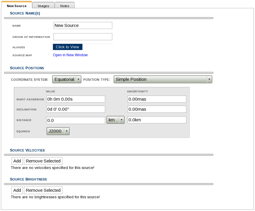 |
| Figure 8.5.1: The New Source screen in the Source Configuration Tool (SCT). |
There are now two choices for setting up a solar system source:
- Sources known internally to the VLA software system, or;
- Sources for which you can provide an ephemeris file.
Note that in the near future you will be able to specify the motion terms of a polynomial, but that is not implemented in the OPT yet.
Internal Sources
For the planets, the software system of the VLA uses an internal representation of the JPL DE410 ephemeris. The list of bodies supported in this way are:
- Sun
- Moon
- Mercury
- Venus
- Mars
- Jupiter
- Saturn
- Uranus
- Neptune
Please note that the positions for the objects specified in this way are barycentric, not bodycentric. The latter introduces small offsets to the actual on-the-sky positions for the VLA. If this is an important effect, you must use the other method of setting up your moving source. When in doubt whether this is affecting your observations, read on about the JPL Horizons page below or consult the NRAO Helpdesk.
To set up an internal ephemeris source, go to the SOURCE POSITIONS section of the New Source page (seen in Figure 8.5.1), and select Solar System Body with Internal Ephemeris in the POSITION TYPE pull-down menu. You will then see something similar to Figure 8.5.2 for the SOURCE POSITIONS section. You can now choose the object from the above list in the SOLAR SYSTEM BODY pull-down menu.
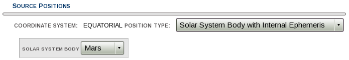 |
| Figure 8.5.2: The SOURCE POSITIONS section for internal ephemeris sources. |
Ephemeris File Sources
If your body is not included in the list of sources known to the VLA, or if you care about bodycentric vs. barycentric positions, you may use an ephemeris file to specify the position of your source as a function of time. To set up an ephemeris file source, go to the SOURCE POSITIONS section of the New Source page (seen in Figure 8.5.1), and select Solar System Body with Uploaded Ephemeris in the POSITION TYPE pull-down menu. You will then see something similar to Figure 8.5.3 for the SOURCE POSITIONS section.
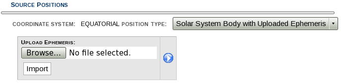 |
| Figure 8.5.3: The SOURCE POSITIONS section for ephemeris file sources. |
Click on the Browse… button to select the ephemeris file, and then click the Import button. The SOURCE POSITIONS section should now look similar to Figure 8.5.4, with the times and positions displayed.
 |
| Figure 8.5.4: The SOURCE POSITIONS section after import of an ephemeris file. |
Format of Ephemeris Files
Ephemeris files to be used in this way are created with the JPL Horizons system. Go to: http://ssd.jpl.nasa.gov/horizons.cgi, and specify:
| Ephemeris Type [change]: | OBSERVER |
| Target Body [change]: | <your source> |
| Observer Location [change]: | GEOCENTRIC [500] (<- "[500]" is part of the location and defines geocentric) |
| Time Span [change]: | <your time range> |
| Table Settings [change]: | QUANTITIES=1,20; extra precision=YES |
| Display/Output [change]: | default (formatted HTML) |
To select your body, click on change next to Target Body, and use the lookup tool. JPL’s Horizons system knows about most solar system bodies, including comets, moons, and asteroids (NEAs included), and even spacecraft. To select your time range, click on change next to Time Span, and input the proper time range. Note that, for most bodies, using an ephemeris tabulated at 1 hour entries is sufficient. For some fast-moving near-Earth objects, a shorter interval between tabulated entries may be needed. To be sure that the Table Settings are correct, click on change, and then be sure that only options (1.) Astrometric RA & DEC and (20.) Observer range & range-rate are selected, then go to the Optional observer-table settings section (below Select observer quantities from table below), and be sure that the extra precision box is checked.
After everything is set up correctly, click on the Use Settings Above button and then Generate Ephemeris.After you are taken to that page, you will need to save the web page as a text file. Please note that currently Google Chrome does not allow for simple saving of web pages as text; Firefox, Safari, and IE do not suffer from this shortcoming. Once the file is saved to your computer, you can select it for use as described above.
Finding Calibrators near Moving Sources
Finding calibrators for moving sources proceeds in much the same way as for other sources, but since the target object moves you must be a bit careful about it. For slow-moving sources in the outer solar system, using the same calibrators over periods of years is fine, since the motion is slow. For inner solar system bodies, however, this cannot be done—each new observation might require a new calibrator, and in extreme cases a single calibrator will not even suffice for a single Scheduling Block (for example, the case of 2005 YU55 mentioned above).
Fortunately, the SCT knows about moving sources, and their locations will be plotted properly in the bulls-eye source plots in that tool. See Figure 8.5.5 for an example. You can either use the normal search cone with radius method of finding a calibrator, or click on the bulls-eye icon for the moving source itself to identify good calibrators. The rules for choosing a calibrator for a moving source are no different than for other sources at the observing frequency.
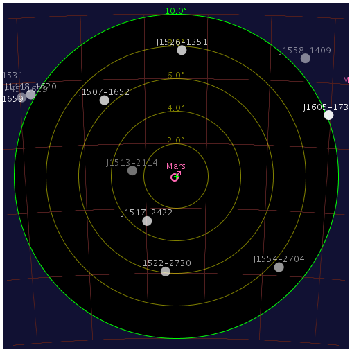 |
| Figure 8.5.5: An SCT bulls-eye plot for a moving source (Mars). |
Solar Observing
Solar Observing
The VLA is able to observe the Sun but it poses a number of challenges: the Sun is a powerful source, it has a complex brightness distribution, it is variable in time – due to solar rotation and due to intrinsic variability (e.g., flares)– and, as a solar system object it displays significant apparent motion on the sky. For these reasons, solar observations require special hardware modifications, different observing procedures, and special calibration software.
The main difference between solar observing and observing sidereal sources from a user perspective is the need to provide one or more ephemerides to ensure that the solar target or targets of interest are tracked. In this respect, solar observing is similar to observing other solar system objects such as planets and comets. Most of the details related to the hardware changes required for solar observing such as switching in the 20 dB attenuators, applying delay corrections, setting stepped attenuator levels, and referring to solar signal to solar Pcal signals are done automatically behind the scenes and are therefore largely invisible to the user.
The OPT is used to produce scheduling blocks (SBs) for solar observations. The basic pattern used for VLA observations applies to solar observations: observation of a bandpass calibrator, and interleaving observations of one or more solar targets with those of one or more gain calibrators. It is assumed here that users are familiar with the OPT and only steps needed to observe a solar source are detailed.
Special Considerations
Array Configurations: The Sun is large, time variable, and can have a complex brightness distribution. It is not advisable to use the A and B-configurations to observe the Sun in general because the uv coverage is simply too dilute. In addition, scattering in the solar corona on density inhomogeneities limits the useful angular resolution with which one can image the Sun. Hence, for most programs, the C and D-configurations are recommended.
Frequency Bands: Solar observations with the VLA are currently available in the L, S, C, X, and Ku bands for which switched-power flux calibration is implemented. They are also possible in P band (230-470 MHz). While P band employed the same 20 dB attenuators to observe the Sun as L, S, and C bands (T302 module) P band does not currently have the special Tcals needed for switched-power flux calibration. Users should be aware that accurate flux calibration is therefore not possible in P band.
Time Sharing vs Subarrays: Solar observers often wish to observe their target in more than one frequency band. It is not possible to do so over a number of days or weeks because solar targets evolve relatively quickly — on time scales of seconds (flares) to hours (active regions). Observers need to carefully consider whether their scientific objectives require observation in more than one band simultaneously, in which case subarrays should be used; or whether they can sample multiple bands in sequence, in which case time sharing is sufficient.
Mosaicking: The field of view of VLA antennas, taken to be roughly the FWHM width of the primary beam, is given as ϑ≈1.5λ arcmin, where λ is the wavelength in cm. For example, while the full disk of the Sun can be mapped with a single pointing for λ=20 cm, one must resort to mosaicking techniques to map the full disk at shorter wavelengths. The current time required per pointing is currently 40-50sec: 20sec to slew, 10sec for setup, and 10-20sec to integrate on source. Hence, users must again weigh desirability of imaging a larger angular domain against the time evolution of emission within the domain over time.
Short Correlator Integration Time (Tint): The Sun produces numerous transient phenomena: jets, flares, radio bursts. For such phenomena, the availability of short time integrations is desirable in order to resolve time scales of interest. The VLA can be used with very short integration times — down to tens of milliseconds. However, the use of short integrations comes at the cost of high data rates and large data volumes. They should be used with caution.
Ultra-high Brightness Sources: At frequencies less than 2-3 GHz, coherent radio bursts from the Sun become increasingly common. They can be highly polarized, show rapid variability (10s of ms), and complex spectral variability. The brightest bursts can exceed 105 solar flux units, or 109 Jy! The VLA 1-2 GHz band has a special signal path (the HNA or "reverse coupler" path) that allows such bursts to be observed without saturating the system. It has not yet been fully commissioned and is therefore not yet available to users. It is anticipated that it will be in the next two years.
Hardware Modifications
The Sun is an extremely intense source of radio emission. To ensure that that the system maintains adequate linearity the solar signal must be reduced to a level that no element along the IF/LO signal chain saturates. Solar observing is currently supported in five of the Cassegrain bands (L, S, C, X, and Ku) and one prime focus band (P band). In the case of the P, L, S, and C bands this is achieved by introducing a switchable 20 dB attenuators into the signal path of each antenna following the first LNA. The attenuator is switched into the signal path in the LSC frequency converter (T302 module). In the case of the X and Ku bands, the 20 dB attenuator is switched into the signal path after the first LNA and postamp. For all bands, the signal is further conditioned in the frequency downconverter which uses stepped input and output attenuators to set optimum signal levels (T304 module).
While the Sun can be observed when the 20 dB attenuators are switched into the signal path, calibrator sources cannot. Hence, the 20 dB attenuators must be switched out of the signal path when observing a calibrator source. The 20 dB attenuators introduce delay into the signal. This delay has been measured for each attenuator in each band and polarization (the attenuator is the same for the L, S, and C bands) and the delay correction is handled online. The stepped attenuators in the frequency downconverter are first optimized on the Sun. If they were allowed to re-optimize on a calibrator source, an uncalibrated phase error would be introduced. Therefore, the stepped attenuators settings are “set and remembered” on the Sun for use during calibrator scans.
Flux calibration is performed using the VLA switched power system (see Perley 2010). Under normal observing conditions a small, stable, and known calibration signal (Pcal) is periodically injected into the signal path following the polarizer at a rate of 20 Hz with a 50% duty cycle. At the point after the signal has been digitally subdivided into subbands, but before it is requantized and correlatated, the system power is synchronously detected when Pcal is switched on and when it is switched off, Pon and Poff. From these, Pdif = Pon - Poff and Psum = Pon + Poff are formed from which the system gain and system temperature can be inferred. From the system gain and the so-called requantizer gain, the cross-power may be calibrated and from thence, the visibility amplitudes.
The VLA front ends have remarkable dynamic range and this arrangement is sufficient to observe the quiet Sun, active regions, and small flares. Unfortunately, the front end will saturate for large flares with the exception of the 1-2 GHz band (L band) for which special provisions have been made.
Source Information
Ephemerides
The user must provide the solar ephemeris or ephemerides needed to execute a solar observing program. A given ephemeris is used to track a particular feature of interest on the Sun, correcting for the Sun’s apparent motion on the sky and for the Sun’s differential rotation. Instances where more than one ephemeris is needed are:
- Time sharing between multiple solar targets.
- The use of subarrays to observe a solar target in more than one frequency band.
- The use of mosaicking to map an angular domain on the Sun that is larger than the primary beam.
Observers may wish to generate their own ephemeris using the JPL Horizons website at http://ssd.jpl.nasa.gov/horizons.cgi (please see the Observing Guide regarding Moving Objects for details). Alternatively, a convenient solar ephemeris generator can be found at http://celestialscenes.com/alma/coords/CoordTool.html. Please read the user manual carefully before using. As its name implies, the ALMA Solar Ephemeris Generator was developed as a tool in support of solar observations with ALMA. However, it can be used to generate ephemerides for solar observations from other observatories, including the VLA.
The ALMA Solar Ephemeris Generator offers two interface choices: GUI or Text. The former is attractive because it allows the user to point and click on solar targets using a user-selected Solar Dynamics Observatory Atmospheric Imaging Assembly reference image or a user-provided reference image. The latter requires the user to specify the helioprojective coordinates of the target.
- Note 1: Unlike ALMA solar observations, VLA solar observations use ephemerides that are referenced to the geocenter, not the location of the array. The reference is specified in the Location field. Click the Change default location (ALMA) box and use the pull-down menu to the right to select geocenter (not VLA!) as the location to which the ephemeris will be referenced.
- Note 2: If using the GUI, do not use the Mosaic observation option in the Pointing field. It is designed for ALMA mosaicking. Instead, generate one ephemeris per VLA mosaic pointing as described in the previous section.
The remaining fields are largely self-explanatory. Upon generating a given ephemeris, the user can inspect the result. If it is satisfactory, it may be downloaded for import into the OPT.
SB Setup
Observers can structure their SBs in the usual way with the following exceptions:
- For a solar SB the first scan must always slew to the Sun. This slew can be used to set attenuators for a dummy resource that uses the same receiver as the actual science resource.
- Once on the sun, observers must use setup scans for each frequency band that will subsequently be used. This ensures that the stepped attenuators in the frequency downconverter are appropriate, i.e., set and remembered.
- For each source thereafter, there should be a scan that slews to the source using the dummy resource, followed by a 10sec setup scan using the science resource to set the requantizer gain (use the setup intent), followed by an observation (calibrate complex gain, calibrate bandpass, calibrate delay, or observe target intents). That is, each source observed — calibrator or target — should be comprised of a triplet of scans that slews, sets up, and observes with the appropriate scan intent(s).
- Note: In cases where a preceding scan uses a different receiver, the requantizer scan length should be 30sec long to account for sub-reflector rotation.
Example
05m00s SOL mode, slew to Sun with dummy resource [intent: setup intent]
01m00s SOL mode, attenuator setup scan on Sun with science resource [intent: setup intent]
02m00s STD mode, slew to phase cal with dummy resource [intent: setup intent]
00m10s STD mode, requantizer setup scan on phase cal with science resource [intent: setup intent]
03m00s STD mode, phase cal scan with science resource [intent: calibrate complex gain (A and P)]
02m00s SOL mode, slew to Sun with dummy resource [intent: setup intent]
00m10s SOL mode, requantizer setup scan on Sun with science resource [intent: setup intent]
Begin Loop (repeat scans n times)
 02m00s SOL mode, observe Sun with science resource [intent: observe target]
End Loop
02m00s STD mode, slew to phase cal with dummy resource [intent: setup intent]
00m10s STD mode, requantizer setup scan on phase cal with science resource [intent: scan intent]
01m20s STD mode, phase cal scan with science resource [intent: calibrate complex gain (A and P)]
04m00s STD mode, slew to flux cal with dummy resource [intent: setup intent]
00m10s STD mode, requantizer setup scan on flux cal with science resource [intent: setup intent]
03m00s STD mode, flux cal scan with science resource [intents: calibrate flux, calibrate bandpass]
Solar SBs, like those of other programs, can be complex and setting them up manually in the OPT can be tedious. It is often advantageous to import an SB or to import scans from an external text file. This is done through, e.g., FILE → IMPORT SCANS whereupon a window pops up prompting the user to Choose File and to Import. It is important to conform to the format expected for an SB or scan import as detailed in Section 5 of the OPT manual.
Calibration
As noted above, flux calibration of solar observations requires use of the switched power system described by Perley (2010). Flux calibration using the switched power system requires calibration in the Astronomical Image Processing System (AIPS). The decision to support flux calibration in AIPS was made as a matter of expediency – implementation in CASA will eventually take place but CASA development has a long lead time. Hence, the recommendation is for users to calibrate their data in AIPS, after which either AIPS or CASA may be used to image the calibrated data.
Calibration of solar data in AIPS proceeds in much the same way that it does for non-solar sources. The one exception is that instead of using the task TYAPL to apply switched power calibration to visibility data, solar observers must use the task SYSOL, which recognizes solar Tcal values for those antennas outfitted with solar Cal sources.
VLBI at the VLA
Introduction
The collecting area, receiver suite, and geographical location of the NRAO's Karl G. Jansky Very Large Array (VLA) make it a valuable addition to a VLBI array. The VLA supports standard VLBI observations at frequencies of 1.7, 3.0, 5.0, 8.4, 15, 22, 33, and 43 GHz. The VLA can take part in VLBI observations as a phased array (Y27). Alternatively, assuming the full collecting area of the phased array in not needed, a single VLA antenna (Y1) can be added to the VLBI observations to provide a short baseline (~50 km) to the Pie Town VLBA antenna.
In phased array mode the VLA offers the equivalent sensitivity, including sampling losses, of a single 115-m antenna. The VLA records up to 4 Gbps to a Mark6 recorder. The time and frequency standard is a hydrogen maser. The VLA participates in High Sensitivity Array (HSA) and Global programs. Its participation must be proposed through normal channels and is arranged by the VLA/VLBA scheduler who can be contacted through schedsoc@nrao.edu. Unless for specific reasons, the data should preferably be correlated at the DiFX correlator located at the Science Operations Center in Socorro, NM.
A well phased VLA, with all 27 antennas, when added to the 10 antennas of the VLBA, will improve the sensitivity in a naturally-weighted image by a factor of about 2.4. Baselines between the phased array and any VLBA antenna should be about 4.6 times more sensitive than baselines between any two VLBA antennas. The addition of the VLA also provides one shorter baseline (Y27-PT) than the VLBA which may be valuable for larger sources.
Questions and concerns should be directed to the NRAO Helpdesk.
Phasing the VLA
TelCal, a real-time program, runs at the VLA during the observations deriving the delay & phase corrections for each antenna/polarization/subband. The antenna signals are then corrected in the correlator, summed up, re-quantized to 2-bits, and finally recorded in VDIF format on the Mark6 recorder at the VLA site.
TelCal does not determine the correction until the end of a scan. In practice, there must be at least 3 good subscans, on a sufficiently strong source, to determine the corrections. The user should allow a scan of about 1 minute for phasing (software run by the NRAO analysts will automatically generate subscans), and the corrections will be determined and stored after the 3rd or 4th subscan. Subsequent scans can apply the stored corrections, e.g. on a target which is too weak to determine the correction.
Autophasing should be done on a calibrator which is a point source to the VLA's synthesized beam and, if transferring phases to a target, close to the target. The strength required depends on the frequency, weather and elevation. A good rule of thumb is >100 mJy for 1-12 GHz and >350 mJy for 12-45 GHz. Higher flux densities are required for low elevations particularly at high frequencies. A good place to look for an autophase calibrator is the VLA calibrator list. For a more interactive search of the VLA calibrator list, we recommend using the Source Catalog Tool (SCT) located in the VLA's Observation Preparation Tool (OPT) suite. The OPT manual provides instructions on how to search for sources in the SCT.
Autophase corrections are valid for a duration that depends on the VLA array configuration, observing band, weather, elevation and, e.g., activity level of the sun. The weather and elevation are particularly important for higher frequencies, and solar activity at lower frequencies. Unfortunately the weather and solar activity cannot really be predicted for these fixed date observations. Our advice is to be conservative because an observation that does not contain frequent enough autophasing cannot be fixed in post-processing for the VLBI data, and sensitivity will be lost. When anticipated at the proposal stage, proper planning can mitigate the effects of weather. Consider observing at night when the atmosphere tends to be calmer and solar activity is not an issue, observing in the winter, and avoiding observing at sunrise and sunset. Very broad rules of thumb for frequency of determining and applying new autophase corrections are:
- C & D config: 20-30 minutes at low frequencies; 10-20 minutes at high frequencies
- A & B config: 5-10 minutes at low frequencies; 2-5 minutes at high frequencies. May want to avoid observing at 45 GHz in these configurations, also because of the very small synthesized beams.
Phasing corrections must also be determined again if you slew to a new part of the sky. In practice, this often means that you have to phase up every time you slew to a fringe finder scan, and again right after each fringe finder when you slew back to the target source. Another broad rule of thumb:
- Low frequency: if you slew to a source more than 15 degrees from the last phasing source, you need to phase up again.
- High frequency: if you slew to a source more than 10 degrees from the last phasing source, you need to phase up again.
Restrictions on Phasing
We are still commissioning the phased VLA so there are some restrictions on phasing:
- Phasing uses all but the edge channels, i.e., a continuum source is assumed.
- Subarrays are not allowed.
- No transfer of phasing between subbands.
- No transfer of phasing across different subband setups. That is, there must be no change in subband setup between determining the phase corrections and applying the phase corrections. Changes in setups include: change observing band, tuning, bandwidth, polarization etc. For example:
- scans 1-6: C-band determine autophase
- scans 7-12: X-band determine autophase
- scan 13: C-band apply autophase
- scan 14: X-band apply autophase
- scan 15: C-band apply autophase
- scan 16: X-band apply autophase
- etc...
- scans 1-6: C-band determine autophase
- scan 7: C-band apply autophase
- scan 8: C-band apply autophase
- scans 9-14: X-band determine autophase
- scan 15: X-band apply autophase
- scan 16: X-band apply autophase
- etc...
- You cannot have a set of scans like this:
- Instead you should have a set of scans like this:
Basebands and Subbands for Phased VLA
For the VLA, "baseband" refers to the frequency band that comes out of the samplers at the antenna electronics racks (its meaning is different from the traditional VLBA baseband). Only 8-bit samplers are used, i.e. there are two 1 GHz basebands, however the entire 1 GHz will not be available for phasing. See the VLA Observational Status Summary for a description of available frequencies and tuning restrictions, but note that they are less restrictive than VLBA tuning limitations.
For the VLA, "subbands" are the continuous blocks of frequency which are correlated by WIDAR and written to the Mark6 unit for VLBI. Two subband pairs (RCP and LCP) may be phased up. Each pair is a different baseband/IF pair AC or BD. So each pair is independently tunable in frequency. Four or 8 subband pairs are also offered as shared risk observing as DDC-8 or PFB modes respectively. See the section on the RDBE in the VLBA OSS for more details on the DDC-8 and PFB modes and their restriction. The subband(s):
- The VLA is always dual polarization, even in shared risk modes. A & C (i.e. RCP and LCP) must be the same frequency and B & D (again, RCP and LCP) must be the same frequency.
- Must have the same bandwidth.
- Bandwidths of 16, 32, 64 and 128 MHz are allowed on a non-shared risk basis. Bandwidths of 1, 2, 4 and 8 MHz have not been tested and are only allowed as shared risk.
- Must align, in frequency and width, with the VLBA IF pairs.
- The restrictions are fewer for the VLA than for the VLBA or other HSA stations, so please follow the HSA guidelines.
- The VLA must be set up to match the VLBA, mixed modes are not allowed.
Given the above restrictions, the maximum bandwidth is 512 MHz in 2 polarizations, which matches the maximum bandwidth on the VLBA. Given 2 bit sampling as on the VLBA, this gives a maximum data rate of 4 Gbps. Observing with the VLA that does not exactly mimic the VLBA in frequency setup is only available under the VLBA Resident Shared Risk Program. Examples of such RSRO projects would be single polarization observing and observing with the full VLA bandwidth but only recording the smaller bandwidth to be compatible with the VLBA.
Scheduling
All phased array observations will be fixed date. Please see the HSA, GMVA, and Global cm VLBI chapter of the Guide to Observing with the VLBA.
Phased array observations will be scheduled in the SCHED program, which is available via anonymous ftp, as described in the SCHED User Manual. Please see the Guide to Observing with the VLBA: Building a Scheduling File in SCHED. A keyin file is used to describe the observation and SCHED processes this keyin file and produces files to run the participating telescopes and correlator. One of the files created by SCHED is the VEX (VLBI Experiment) file which describes the entire observation. There is a program called vex2opt which converts the VEX file into files that can be read in by the VLA Observation Preparation Tool (OPT). Vex2opt will be run by NRAO staff once the schedule is submitted. The OPT will then write the observing script for the VLA.
Standard practice is for the user to send the SCHED keyin file to vlbiobs@lbo.us, NRAO staff will then run SCHED, and distribute any control files to the telescopes participating in the observation. They will run vex2opt and submit the VLA script. However, the user may edit the VLA schedule after it is loaded into the OPT. If the observer adjusts the VLA schedule and the observation fails because of that, then the fault lies solely on the observer and there is no requirement of the NRAO to offer a remedy. Note that SCHED can schedule VLA specific items like pointing, flux calibration, etc., so there is little reason to modify the VLA schedule in the OPT.
The observation will also produce standard VLA visibility data, so the user will probably want to do standard VLA flux calibration, and other calibration required to use the VLA data by itself.
If you have problems scheduling or anything else please use the NRAO Helpdesk.
Log Files
After the observation is over the observer will receive by email logs from the VLA operator and the VLBA operator.
Frequencies
Please see the VLA and VLBA Observational Status Summary (OSS) for specifics on frequency ranges and tuning limitations. Generally the VLBA is more restricted than the VLA, so it would be best to start with the VLBA. The VLA and VLBA have similar frequency bands, but the VLA receivers generally have a wider tuning range. The common frequency bands are: L (1.35 - 1.75 GHz), S (2.15 - 2.35), C (3.9 - 7.9), X (8.0 - 8.8), Ku (12.0 - 15.4), K (21.7 - 24.1) and Q (41.0 - 45.0). Currently P-band (0.23-0.47 GHz) cannot be phased.
VLA Modes
Both phased array (Y27) and single VLA dish (Y1) can be used. For situations where the observer may only want the inner antennas of the whole VLA to be phased up, a comment to the operator would suffice . All antennas in the subarray will be used for phasing, and all will be included in the phased sum. For instance, you cannot obtain WIDAR correlations for all antennas but use only a subset of those antennas in phasing or in forming the phased sum for VLBI recording.
There are also two basic modes when scheduling the phased array: determine autophasing and apply autophasing.
Data from the VLA
The VLA will produce two sets of data: 1) VDIF format data written to Mark6 recorder intended to be correlated with VLBA; and 2) standard WIDAR (VLA) correlator output.
The standard WIDAR (VLA) correlator output will be available from the NRAO data archive and can be accessed through the observer's my.nrao.edu account. This data will be 64 channels per subband per polarization product and have a 1 second integration time (regardless of configuration).
Practicalities
When preparing VLA schedule files, the following facts and guidelines should be noted:
- Please see the HSA/GMVA/Global VLBI and Building a Scheduling File in SCHED chapters of the Guide to Observing with the VLBA.
- The observer should follow the VLA general observing restrictions and advice, such as the one minute setup scan for each correlator configuration (i.e. band) at the beginning of the observation and the amount of overhead needed for reference pointing at the start of an observation.
- As a rule of thumb, the source on which you autophase should be a point source (to the VLA's synthesized beam) with >100 mJy for 1-12 GHz and >350 mJy for 12-45 GHz. Note that stronger sources may be required in bad weather and/or low elevation, particularly for higher frequencies.
- Assume about 1 minute to determine autophase.
- The frequency of determining/applying a new autophase depends on the VLA array configuration, elevation, day or night observations, the observing band and the weather. Please see the Phasing the VLA section for more details.
- Subarrays are not allowed.
- No pulse calibration system is available at the VLA. If you plan to use more than one subband, then you should observe a strong and compact source to serve as a manual pulse calibrator; see the VLBA Observational Status Summary.
- The minimum VLA elevation is 8°. The maximum VLA elevation is 125° if over-the-top antenna motion is allowed by the observer. However, such antenna motion is not normally recommended and not the default. At zenith angles less than about 2°, source tracking can be difficult.
- Positions accurate to a VLA synthesized beam (rather than the much larger primary beam) must be used for phased-array observations.
- Strong radio frequency interference (rfi) can make it impossible to autophase, so pick your subbands to avoid rfi.
- Those using the VLA at frequencies higher than 15 GHz should be aware that antenna pointing can be poor at these wavelengths. Therefore at these frequencies reference pointing for the VLA should be used, again see VLA documentation on high frequency observing.
- If you want to derive source flux densities and/or produce images from the standard VLA data, then your VLA observe file should include at least one scan of a flux density scale calibrator for the VLA.
- The VLA slews at a slower rate than the VLBA.
- If you want to do polarimetry with the standard VLA's data please consult the Polarimetry section of the Guide to Observing with the VLA.
Questions and concerns should be directed to the NRAO Helpdesk.
Pulsars
Introduction
The VLA is capable of performing imaging observations of pulsars by "phase-binning" visibilities (also sometimes known as gating). In this observing mode, rather than continuously integrating visibility data for several seconds as in a standard observation, the data are accumulated into a number of "bins" corresponding to different rotational phase ranges of the pulsar. The predicted phase versus time is computed from a user-supplied pulsar timing ephemeris; see below for more details. This allows each pulse phase bin to be imaged separately, for example to identify which continuum source in a given field is the pulsar, or to image the surrounding area after subtracting off pulsed emission, or simply to increase S/N on the pulsar relative to a standard image, etc.
Note that this mode is not suitable for observations of pulsars whose period is unknown a priori, or for observations of single pulses from sources such as FRBs or RRATs.
Correlator Setup
There are several constraints on the bin width, total allowed bandwidth, and data rate that are specific to pulsar binning observations. These are described in detail in the OSS pulsar section and in the VLA proposal guide. Once you have decided on your basic setup (band, frequency resolution, etc), set up the subbands following the general instructions given in the RCT manual. Pulsar binning can then be enabled by going to the "Pulsar" tab in the RCT, selecting "Phase Binned Imaging" mode, and entering the number of bins, as shown in Figure 8.8.1 below:
 |
| Figure 8.8.1: Setting Pulsar Mode for resource |
The final option specifies whether the pulse period model should be computed from a timing ephemeris, also known as a "par file" or alternately if the binning should be done at a constant topocentric pulse period. The RCT will verify that the chosen configuration is possible, and will report the total data rate, as shown.
Calibration
In general there is no special calibration that needs to be done for binning observations. Calibration procedures for complex gain, flux density scale, and if necessary polarization should follow the general guidelines laid out in the Calibration section of the manual. The only notable differences for pulsar observing are:
- Calibrators should be observed using a standard (non-binned) correlator setup. It is recommended that this setup use the same frequency configuration (tuning frequencies, subbands, numbers of channels) as is used for your pulsar target. The easiest thing to do is first set up the pulsar configuration, then make a copy of it in the RCT and disable binning.
- As for all VLA observing, binning projects should include an initial setup scan for each band used, to set attenuator levels. However, there is no need to include additional setup scans to trigger requantizer setting.
Pulsar Ephemerides
When observing pulsars the apparent pulse period is slowly changing with time due to a number of effects including motion of the Earth, motion of the pulsar (binary orbits), intrinsic spin evolution, etc. The period versus time can be predicted using an ephemeris or timing model. For binning observations, you should supply an ephemeris using the standard TEMPO "par file" format. A polynomial approximation to the pulse phase versus time will be generated on the fly using TEMPO at the time of your observation and used for binning the visibilities. Note that TEMPO2-format par files are not currently accepted. If you have a par file in TEMPO2 format (for example if it includes "UNITS TCB"), you will need to convert it to TEMPO (TDB) format.
Pulsar ephemerides should be uploaded into your source catalog in the SCT via the "Pulsar Ephemeris" (Figure 8.8.2):
 |
| Figure 8.8.2: Pulsar Ephemeris tab |
Since VLA binning observations always generate bins covering the full pulse period there is no need to have absolute phase information about the source you are observing. This also means it is not strictly necessary that the ephemeris be accurate over the full length of your observation, although the pulse "drifting" into different bins versus time may make data analysis harder. The fundamental requirement to avoid smearing out pulses is that ΔP x δt < 1/Nbin, where ΔP is the error in the predicted pulse period and δt is the correlator integration time.
Many pulsar ephemerides can be found in the ATNF Pulsar Catalog, but they are not necessarily up to date for all sources. It is always worthwhile to verify a timing model with recent data if there is any uncertainty about it.
Flux Density Scale, Polarization Leakage, Polarization Angle Tables
3C48
# 3C48
# Date 31Jan/01Feb 2019 polarization properties
# Reference flux densities were used
# Frequency  I       P.F.       P.A.
# (GHz)      (Jy)               (rad)
1.022        20.68   0.00293     0.07445
1.465        15.62   0.00457    -0.60282
1.865        12.88   0.00897     0.39760
2.565        9.82    0.01548    -1.97046
3.565        7.31    0.02911    -1.46542
4.885        5.48    0.04286    -1.24875
6.680        4.12    0.05356    -1.15533
8.435        3.34    0.05430    -1.10638
11.320       2.56    0.05727    -1.08602
14.065       2.14    0.06097    -1.09597
16.564       1.86    0.06296    -1.11891
19.064       1.67    0.06492    -1.18266
25.564       1.33    0.07153    -1.25369
32.064       1.11    0.06442    -1.32430
37.064       1.00    0.06686    -1.33697
42.064       0.92    0.05552    -1.46381
48.064       0.82    0.06773    -1.46412
Link to download 3C48_2019.txt file.
3C138
# 3C138
# Date 31Jan/01Feb 2019 polarization properties
# Reference flux densities were used
# Frequency  I       P.F.       P.A.
# (GHz)      (Jy)               (rad)
1.022        10.07   0.05462    -0.23182
1.465        8.26    0.07795    -0.16694
1.865        7.21    0.08955    -0.16235
2.565        6.00    0.09848    -0.17721
3.565        4.89    0.10337    -0.16619
4.885        4.00    0.10524    -0.18386
6.680        3.23    0.10219    -0.20056
8.435        2.76    0.10939    -0.16412
11.320       2.24    0.09063    -0.13864
14.065       1.90    0.08231    -0.18290
16.654       1.69    0.08186    -0.23086
19.064       1.54    0.08437    -0.28012
25.564       1.25    0.08422    -0.31691
32.064       1.06    0.08541    -0.33910
37.064       0.96    0.08694    -0.34084
42.064       0.88    0.08772    -0.40503
48.064       0.82    0.09147    -0.42097
Link to download 3C138_2019.txt file.
3C147
# 3C147
# Date 31Jan/01Feb 2019 polarization properties
# Reference flux densities were used
# Frequency  I       P.F.      P.A.
# (GHz)      (Jy)              (rad)
1.022        27.73   0.00028    N/A
1.465        21.36   0.00018    N/A
1.865        17.86   0.00021    N/A
2.565        13.79   0.00015    N/A
3.565        10.40   0.00052   -0.59515
4.885        7.88    0.00157   -0.23002
6.680        5.91    0.00514   -1.00103
8.435        4.81    0.00476   -0.33225
11.320       3.67    0.00849    0.46557
14.065       3.02    0.01791    0.91642
16.564       2.61    0.02400    1.04399
19.064       2.32    0.02904    1.14768
25.564       1.82    0.03432    1.37341
32.064       1.53    0.04033    1.43967
37.064       1.38    0.04470    1.52606
42.064       1.26    0.04943    1.51182
48.064       1.14    0.05956    1.48944
Link to download 3C147_2019.txt file.
3C196
# 3C196
# Date 31Jan/01Feb 2019 polarization properties
# Reference flux densities were used
# Frequency  I       P.F.        P.A.
# (GHz)      (Jy)                (rad)
1.022        18.94   0.00048     0.78540
1.465        13.75   0.00052     0.29400
1.865        11.05   0.00174     0.70710
2.565        8.14    0.00992     0.89138
3.565        5.86    0.02256    -1.36438
4.885        4.22    0.02499    -0.97477
6.680        3.00    0.01969    -0.71829
8.435        2.33    0.01602    -0.59490
11.320       1.67    0.01293    -0.51003
14.065       1.30    0.01254    -0.51098
16.654       1.08    0.01244    -0.48004
19.064       0.92    0.01278    -0.57629
25.564       0.66    0.01307    -0.42159
32.064       0.51    0.01165    -0.45858
37.064       0.43    0.00595    -0.26686
42.064       0.37    0.02809    -0.38925
48.064       0.31    N/A        N/A
Link to download 3C196_2019.txt file.
3C286
# 3C286 - values from R. Perley based on 3C286
# Date 31Jan/01Feb 2019 polarization properties
# Reference flux densities were used
# Frequency  I        P.F.        P.A.
# (GHz)      (Jy)                 (rad)
1.022        17.46    0.08618     0.57632
1.465        14.64    0.09794     0.57261
1.865        13.03    0.10122     0.57613
2.565        10.85    0.10575     0.57580
3.565        8.94     0.11153     0.57624
4.885        7.33     0.11525     0.57503
6.680        5.97     0.11858     0.57758
8.435        5.12     0.12045     0.57827
11.320       4.12     0.12261     0.58412
14.065       3.54     0.12303     0.59534
16.564       3.15     0.12544     0.60172
19.064       2.85     0.12633     0.60286
25.564       2.30     0.12700     0.62198
32.064       1.92     0.13062     0.63170
37.064       1.73     0.13485     0.62791
42.064       1.57     0.13420     0.64589
48.064       1.44     0.14629     0.62153
Link to download 3C286_2019.txt file.
3C295
# 3C295
# Date 31Jan/01Feb 2019 polarization properties
# Reference flux densities were used
# Frequency   I       P.F.       P.A.
# (GHz)       (Jy)               (rad)
1.022         29.13   0.00048    0.78540
1.465         21.60   0.00017    N/A
1.865         17.54   0.00045    0.34737
2.565         12.84   0.00047    0.78540
3.565         9.12    0.00102   -1.23511
4.885         6.42    0.00198    1.43111
6.680         4.45    0.00849   -0.10259
8.435         3.37    0.01134    0.54597
11.320        2.33    0.01537   -0.63780
14.065        1.75    0.01372   -1.16634
16.564        1.43    0.02449   -1.53089
19.064        1.19    0.03485    1.38367
25.564        0.82    0.05047    1.06163
32.064        0.60    0.06503    0.88536
37.064        0.50    0.06517    0.74524
42.064        0.44    0.06131    0.79286
48.064        0.41    N/A        N/A
Link to download 3C295_2019.txt file.
Presubmission Checklists
Instrument Validation
Integration Time & Time Averaging
The correlator integration time (Tint) should be appropriate for the array configuration, your scientific goals, and observing mode (i.e., on-the-fly-mosaicking, subarrays). Make sure you have short enough integration time in order to reduce time averaging losses and to offset atmospheric/ionospheric phase winding. The minimum possible integration time depends on the total number of channels produced in the correlator and the maximum data rate and data volume. The smaller the integration time, the larger your data set will be. Thus, making the integration time unnecessarily small should be avoided. Current integration time defaults and guidelines can be found in the Time Resolution and Data Rates section of the current VLA OSS.
Consider that time averaging causes some smearing of sources away from the phase center of the image; the further away from the phase center, the more smearing there is. This effect cannot be remedied by self-calibration and it persists after deconvolution. Therefore, it is important to devise observing strategies that hold the distortions down to acceptable levels. For more details, refer to the Time-Averaging Loss section in the current VLA OSS.
Continuum
Most observers will be able to utilize the NRAO's default continuum resources located within the Instrument Configuration tool (also known as the Resource Catalog Tool (RCT)). When choosing one of the defaults, be sure to select the resource according to the array configuration in which the SB will be observed. The defaults are organized by array configuration and corresponding correlator integration time. For example, A/Any config will contain 2s integration time resources and DCB/Any config will contain 3s and 5s integration time resources.
Did you choose the correct default resource?
While checking the Reports tab of the SB in question, the first table of that page summarizes the resource(s) utilized within in the SB. The NRAO defaults adhere to the following naming scheme: the first letter denotes the receiver band, the number following signifies the total number of subbands, the letter following denotes the polarization (f=full and d=dual), and the last number indicates the correlator integration time in seconds. Some defaults contain extra letters at the end, these signify the preferred array configuration for its integration time.
Default Examples:
K64f2 = K band, 64 subbands (3-bit), full polarization, 2s integration time
X16f5DCB = X band, 16 subbands (8-bit), full polarization, 5s integration time, D, C, or B configuration
The distinction between 3-bit and 8-bit resources can be made through the number of the subbands: 8-bit resources, regardless of the receiver band, have 16 subbands. The 3-bit resources have 64 subbands at K, Ka, and Q-bands, 48 subbands at Ku-band, and 32 subbands at X and C-bands. In order to see a detailed overview of a resource within an SB, click on Show All Subbands located in the first table of the Reports tab.
If a given default resource is not exactly what is required for the science (i.e., the default center frequency is not ideal), then the observer can either create a new continuum resource from scratch or copy/paste a default resource into their own catalog and then make adjustments to the resource as needed.
For very detailed guidelines on how to create continuum and spectral line resources, please read through the section on how to Create a Personal Resource Catalog within the OPT Manual.
Spectral Line
As noted above, please read the section Create a Personal Resource Catalog within the OPT Manual in addition to reading through the Spectral Line section within the Guide to Observing with the VLA.
If you are setting a spectral line resource that requires narrow subbands, you may want to use Doppler Setting. Details on this are available in the Spectral Line observing guide and the Spectral Line Setup of the OPT manual. With velocity resolution, make sure the spectral resolution is enough to resolve your line (take subsequent Hanning smoothing into account) and possibly over-sample by a factor of 4 to be able to correct for Doppler Setting effects. Also, make sure you have enough line-free bandwidth to measure the continuum flux.
During the process of building your spectral line resource be aware if, at the time of line placement, you see the following warning message in the pop up window: Warning: The subband overlaps a forbidden region of the baseband. When this happens, the 128 MHz boundary condition overrules the sky frequency of the subband and the subband gets placed off from the desired value because it cannot be on the boundary itself (note, this process is not reversible). The only way to address this is to shift the baseband frequency (within the Baseband tab).
When you change the baseband frequency, make sure to re-generate the subbands containing the spectral lines which had the above noted warning. The original spectral lines have been forced to a different frequency due to hitting the 128 MHz boundary.(Note, be sure to remove any incorrectly placed spectral lines within the subbands.) Then update the scheduling block (SB) with the new resource, and finally verify that the subbands are as expected in the Reports tab of the OPT (explained below).
After generating the lines, be sure to double check and/or adjust the following parameters to achieve the desired resolution:
- bandwidth (BW)
- polarization: full or dual
- Baseline Board Pairs (BlBPs) stacking
- Recirculation
Spectral Line Validity Check
Once the resource has been created and imported into the SB, we recommend performing a check on the spectral line sky frequencies and Doppler Settings (if applicable) to verify that everything is ok.
- Within the OPT, go to the SB containing the resource in question and then go to the Reports tab. At the top of that page, insert an LST date and start time in the assumed LST start fields, then click Update. (LST dates for a given month can be found on the figure in the Scheduling Constraints page.)
- In the Instrument Configuration Summary table (found within the Reports tab of an SB), locate the resource of interest and find the Doppler line, velocity, position, etc. columns. If they contain dashes instead of values, then the resource has not been set up to apply Doppler corrections at the time of observing and all frequency information for this resource relates to sky frequencies. Assuming Doppler corrections are essential, switch them on in the resource (bottom of the Baseband tab within the Instrument Configuration tool), change the resource name and re-import the new resource to all the scans with the old resource (using the Bulk Edit tab) and check these columns in the resource again.
- Click Show All Subbands for the resource of interest. Here you will see the calculated sky frequencies of all subbands (frequency range, subband center, etc...) for the assumed date of the above step. With Doppler Setting active, these frequencies will change with date and time of observation as they are not fixed sky frequencies.
- Select one of your lines to compare the subband center frequency with the value generated through the Dopset tool. In the Dopset tool, populate the appropriate fields, including the LST day and time you used in the OPT. The frequency reported by Dopset and the OPT may not be identical but it should be very close (within a kHz). However, if Doppler Setting was not used in the resource, then there would be a noticeable difference in the frequencies between Dopset and the OPT. For such cases, make sure that your spectral line of interest is well within the subband even if it is not at its center.
- Repeat step 3 for other spectral lines in both the A/C and B/D basebands.
- Repeat steps 3 and 4 for the other LST start dates/times to make sure the frequency values in the table will change as expected due to Doppler and are consistent with Dopset.
If you have questions or need assistance, please submit a ticket to the NRAO Science Helpdesk and include the URL of the resource in question along with the project code.
SB Validation
In this section we provide practical considerations to ensure that your VLA scheduling block (SB) adheres to the discrete requirements for successful observations. Please follow this list during the preparation of your SB and before submitting it through the Observation Preparation Tool (OPT). If you wish to check the validity of the correlator setup of your observations, please visit the Instrument Configuration Verification page.
It is essential that one checks their SBs carefully prior to submitting. Although the OPT has several features to deal with logistical observing issues, it will not catch everything. The same goes for the SB verification that NRAO staff performs after submission; SBs are checked only for common errors. Items like source positions, Doppler-setting frequencies, choice of calibrators, etc., and anything particular that refers to the science goal of the observations cannot be verified by the staff. Remember that the final responsibility for a correct observing schedule remains with the observer.
Do not observe too close to the Sun, especially at low frequencies. This is not related to selecting the "avoid sunrise/sunset" options within an SB. For more information, refer to the Avoiding the Sun section.
If you would like more help with validating your SB(s) (i.e., instrument configuration or appropriate calibrators), please submit your questions to the NRAO Helpdesk.
Information Tab
- Appropriate wind and API constraints:
- Important because most of VLA observing is dynamic.
- Be aware of selecting "avoid sunrise/sunset":
- In most cases this is not necessary and can decrease the chances of observing. For more details, refer to the Low Frequency and Very Low Frequency strategy guides.
- Duration of the SB:
- This is highly dependent on the observing priority of the SB. Please see the optimal duration question in the Frequently Asked Questions section. (Note, any length of SB is permitted, i.e., 33min, 1hr12min, etc..)
- Count:
- Should the SB be observed more than once?
- LST start range:
- This should be set when all sources are above the VLA's horizon.
- Earliest and Latest UT start date and time:
- This may be set to avoid observing too soon after submission or during a specific date range.
Static Report Tab
- Setup scans:
- These are needed for observations with both the 8-bit and 3-bit samplers. Please see the 8/3-Bit Attenuation and Setup Scans section for more details (note there are special instructions for S- and P-band observations).
- Start-up time:
- This can be 10-14 minutes at the start of the SB. It is primarily for the initial slew to the first source in the SB and for setup scan(s). These are followed by the first calibrator-intent scan for low frequency observations or the first reference pointing scan for high frequency observations.
- Scans in Duration (LST) only:
- In this mode, scans include both slew and on-source time.
- Antenna Wrap Requests:
- While checking the elevation, make sure to set the LST start range to avoid antenna wrap issues and request an antenna wrap when appropriate. Note, not all SBs will require an antenna wrap request.
- Elevation Limits: Ensure that all scans (for all LST start times) have appropriate elevation limits.
- High frequency (> 15 GHz) observing: avoid elevations < 30° (if possible) and > 80° (required).
- Low frequency (< 15 GHz) observing: avoid elevations < 10° (recommended) and > 85°.
- S-band (2-4 GHz) observing: avoid elevations < 20° (recommended to avoid ground spill-over).
- The VLA's hard lower elevation limit is 8°.
- Step through the LST start range to validate elevation limits for all scans.
- Double check the science target source coordinates are correct and are using the J2000 epoch.
- Include all necessary calibrators: complex gain, flux density scale, bandpass (and delay) and, if applicable, polarization.
- Bracket the science target scans with the complex gain calibrator and use the appropriate cycle time: This is especially important for high frequency observing. An exception may be when the target can be self-calibrated. The final decision, however, is up to the observer.
- If observing more than one frequency (LO/IF) setting - this being within a single receiver band or through multiple receiver bands - and switching between them in the SB, there is no guarantee to return to the same phase state upon returning back to a given frequency setting. Therefore, in such cases it is extremely important to bracket the target with complex gain calibrator scans that use the same frequency setting as the target to avoid experiencing any phase jumps.
- All scans have appropriate scan intents: If you wish to use the VLA Calibration Pipeline, a flux density scale and bandpass calibrator must be defined in the SB. (Note, do not use Determine Autophase or apply last Phase & Delay cal; these are reserved only for VLBI observations.)
- Use and apply reference pointing: Interferometric reference pointing is needed during high frequency (> 15 GHz) observing with the solutions applied to the proceeding scans. For more details, see the Antenna Reference Pointing Calibration section in the Calibration guide.
- Repeat reference pointing scans when the difference from the last pointing position is at least 20° on the sky in AZ or EL.
- Minimum on source time: [On the Reports tab of the SB, step through the LST start range to verify sufficient on source time.]
- For regular (standard observing) scans, no less than 20 seconds on source after slewing. Note that the OPT will assume a minimum slew time of 20 seconds, including "slew" between receiver bands (to rotate and focus the subreflector). This 20s however is too short when P-band and L-band or S-band are involved. For switching between these bands (P↔L or P↔S) add another 15s for the"slew" and thus anticipate a minimum of 35 seconds on source as reported on the Reports tab.
- For flux density scale calibrator (standard observing) scans, no less than 40 seconds on source after slewing.
- For reference pointing scans, no less than 2.5 minutes on source after slewing.
- Maximum total scan length: [In all cases, be sure to adhere to the recommended calibrator cycle time.]
- Regular (standard observing) scan types may be up to 30 minutes in total duration. However, we highly recommend using a sequence of shorter scans to avoid significant loss of data if a scan is dropped during the observation.
- OTF mosaicking scans are not subject to a maximum scan duration limit.
- Interferometric pointing (reference pointing) scans, under practical terms, can be as long as needed to ensure the required minimum 2.5 minutes of on-calibrator time.
Dynamic LST Validation Tab
This is a new tab created to help observers check their SBs more thoroughly for time on source, elevation limits, antenna shadowing (for D and C-configuration only), and other parameters. For a detailed overview, please refer to the Dynamic LST Validation section of the OPT manual.
Frequently Asked Questions
Observing with a certain cadence (e.g., weekly or monthly)
The Proposal Submission Tool (PST) allows the proposers to request a given observing session to be repeated with a certain cadence (e.g., observing once a week to monitor a source). However, this information does not propagate to the Observation Preparation Tool (OPT). Furthermore, the OPT itself does not have a built-in mode to support such observations. Therefore, it is the observer's responsibility to keep track of the observations and ensure they take place with the desired cadence.
To illustrate this, consider the scenario that a given SB needs to be observed 5 times with a one week cadence. The observers have the following two options:
Option A: Submit one SB at a time with an earliest UT start date clearly marked under the Information tab in the OPT. The observer keeps track of when it is observed and then submit the next SB in the cadence (with the next earliest UT start date), and so on.
Option B: Submit five single-count SBs each with an earliest UT start date set one week apart from each other. The observer keeps track of when the SBs are observed, cancel the submissions of any SBs if/when needed to reset the earliest UT start date and resubmit in order to keep with the cadence. The earliest/latest UT start date/time can be adjusted in an SB without unsubmitting.
Note that requesting the observation of a given SB for a given day does not guarantee its execution; this is dependent on the scientific priority of the project and the dynamic scheduling conditions (such as weather).
For both options A and B we also require the following information: In each SB the observers need to add a comment to the operator (the text box under the Information tab) clarifying the earliest UT start date with the local date, e.g., "Observe Friday evening Mar04 local / Mar05 UT at the earliest". This is because the Observation Scheduling Tool (OST) of the VLA can sometimes select an SB a day earlier than the earliest UT start date. However, note that the array operators will not keep track of when an SB in a cadence should be observed or unsubmitted. This responsibility is entirely on the observer.
What are linked SBs and how do I make them?
Occasionally you may need to prepare and submit more than one version (sometimes two or more) for a given SB. The need to submit multiple SBs may result from antenna wrap issues as well as the need to observe certain critical calibrators that are attempting to compete for the same allocated time; i.e., if one of the SBs are observed then the others will not be needed. We refer such multiple SBs as "linked" SBs.
Preferred Method of Creating Linked SBs
The OPT can now use conditional formatting to create, among other options, linked SBs. The OPT manual has documentation on how to use conditional formatting to create linked SBs and below is given a quick overview on how to use conditional formatting to create linked SBs. The conditional formatting is set at the Program Block (PB) level of your project.
- You will see a section before the table with your SBs that is titled "Linked Scheduling Blocks"
- You enter the INDEX number (not the SB ID) of the SB(s) that you want to have conditional formatting run on. These are entered in the "Block Indicies" field in the format index_id (,index_id,...), e.g. 1,2,...
- Select from the drop down at left either "Any of the observations" or "One of the observations"
- Select the type of conditional formatting, Time (repeat the SBs in the list until a set number of hours is reached) or Executions (repeat the SBs until a set number of executions has been reached)
- Click on "Add" button then "Stop Editing Constraints" button to apply the conditional formatting
For example, linked SBs where you want only 1 of the pair (or more for multiple linked SBs) to be executed would be: Any of the observations, index_ids of the SBs, Executions = 1 (or more if the SBs have a count > 1)
You can add multiple conditional statements and they are executed from top down, and you can reorder the sequence of conditional formatting.
You can also use conditional formatting to prioritize which SB(s), all other factors being equal (e.g., wind and API constraints, SB length, LST time range, etc.), should be considered first for observing.
|
Figure 10.1: Conditional Format statement to accumulate multiple observations based on a maximum time. Note that the SBs that correspond to the SB Index number may need to have a count > 1 if they are shorter than the maximum time and you want them to repeat observation. |
|
Figure 10.2: Two Conditional Format statement to observe only one SB in a list of SBs. Note that the statement is evaluated from left to right so that, all things being equal, the leftmost SB will be selected over the rightmost SB. (Note: the blue color is due to the format being selected when the capture was made.) |
|
Figure 10.3: Conditional Format statement for multiple observations. With this statement the SBs require counts > 1. In this way you could have SB Index 1 run up to 3 times or SB Index 2 run up to 3 times or a mix of runs of SB Index 1 and 2 (e.g., SB Index 1 run twice, SB Index 2 run once or vice versa). |
Important notice when removing SBs from a Conditional Format list.
If an SB is removed (i.e., cut from the left-hand column list), the indexing of the SBs will be renumbered. Therefore, all linked SBs should be double-checked in case the renumbering of the SB index affected those linked SBs. If those linked SBs received new indexes, then the conditional format should be removed and a new conditional format be added. If a linked SB is unsubmitted, the conditional format with the SB index will be automatically removed. Be sure to re-link the SBs.
Old Method of making Linked SBs (DO NOT USE)
The 'Comment to the operator' field under the Information tab of the SB in the OPT, a comment is entered that makes the operator aware that this SB is linked with other SB(s), and if the current SB is executed on the array to not execute the other SB(s) linked to it. The major caveat is the operators often do not see these comments and rely on their scheduling tool to place linked SBs on hold automatically. Therefore, please use the preferred method of linking SBs as described above.
What is the optimal duration of my Scheduling Block?
How does the duration of my scheduling block affect the probability that it will be observed?
This depends strongly on the priority (A, B, or C) assigned to your project:
A-priority: dynamic scheduling enables priority A projects to observe during the requested observing conditions as determined at the start of the observation. Scheduling blocks of any length are fine as far as the heuristics in the dynamic scheduler are concerned. However, there may be other considerations in determining the best SB length. At the start of any observation the phase stability constraint given in the scheduling block gets evaluated. For high frequency observations, and even if at the start of the observations the phase stability was adequate, it may degrade with time due to changing weather conditions. Therefore, the degradation of the phase stability across long duration observations (greater than 2+hours) is a factor that needs to be taken into consideration by the observer. This degradation is a function of both time of day and time of year. Phase stability can not be guaranteed for long duration SBs.
B-priority: the number of priority B projects approved is designed to fit into the available hours per configuration, but shorter SBs (4 hrs or less) help with scheduling around priority A projects.
C-priority: these are filler projects, and only short SBs (ideally 0.5 to 1 hr in length, certainly no longer than 2 hrs) have any chance of getting observed.
What integration time should I use?
The default integration times for bands per array configuration can be found in the Time Resolution and Data Rates Section of the OSS. For reference pointing scans, the integration time should always be 1 second, regardless of band and array configuration.
How long does an antenna reference pointing calibration scan need to be?
Antenna reference pointing calibration needs a scan with an on-source time of 2m30s in addition to any slew time.
What is the difference between Doppler Tracking and Setting?
Doppler Tracking, the automatic adjustment of the sky frequency from scan to scan, is not supported in VLA observations. Since start date and time of the observation are unknown, manual Doppler tracking (calculating and entering sky frequencies manually for each scan) is not an alternative. The user is advised to use one sky frequency per source for the duration of the scheduling block. If the diurnal variation (up to 1 km/s) exceeds a certain fraction of the channel width, the data need to be re-sampled along the frequency axis during post processing. For this to work, make sure that at the time of observing the data are sufficiently oversampled in frequency to avoid artifacts from the re-binning to affect the data.
Doppler Setting - The Earth's orbital motion around the sun can cause changes in velocity of up to 60 km/s in the course of a year, potentially shifting the line outside the available band. The VLA's Observation Preparation Tool (OPT) supports Doppler Setting. For each Doppler Setting resource, the sky frequency is calculated at the start of the observation and kept constant for that source during the observation. This precludes the earlier requirement to periodically resubmit Scheduling Blocks with updated sky frequencies. For more information on Doppler Setting, see the Spectral Line section.
If Doppler Setting is not selected, the observer will have to calculate the sky frequency manually using the Dopset Tool, entering an estimate for the observing date.
Should I observe source and calibrator at the same frequency?
We strongly recommend against transferring phases from (complex gain) calibrator to source when each is observed at a different frequency; an exception would be for Galactic HI studies. Therefore, if sources are observed at more than one frequency, make sure to bracket each source scan with the complex gain calibrator scans at the same frequency as the source scan. For the same reason there also should be a separate flux density and bandpass scan for each frequency.
How do I change an instrument configuration in my SB?
I have made a scheduling block using a certain Instrument Configuration and I want to change that configuration. Is that all I need to do?
No. Sources and Instrument configurations become part of the scheduling block at the time you specify them in a scan. Changes to sources or instrument configurations in the SCT or RCT therefore do not automatically propagate to the scheduling block. To apply such a change to an existing scheduling block open it and use the Bulk Scan Edit tab available on top of the right hand panel.
Also, to be absolutely sure that the changes have taken effect, check again the Reports tab of the scheduling block. The resources table (the table directly below the information at the top) should reflect the change and not have a single scan with the old resource values which should not appear if all scans were updated. The easiest way to see this is to give your modified or new resource a different name, then the only check is to see if the new resource name is listed as a resource in the table and the reference to the old name has gone. This is, of course, less straight forward for a source if a position is updated; for a change in sources check the sources table (between the resources table and scan table) very carefully for your edits.
What happened to Fast Switching?
I used to use fast switching for my high frequency observations with the old VLA. Is there something similar on the current VLA?
Fast switching used to be a special mode in the old VLA because, compared to specifying the individual scans, it saved on overhead and therefore made more efficient use of observing time. With the current online system there is no such penalty, precluding the need for a fast switching mode, the functionality of which is now fully covered by scan loops. For more information, see the Scan Loops section of the OPT Manual.
Are there any tuning restrictions for the IFs?
General:
- For very wide frequency separations at K, Ka, or Q band, IF pair B/D (i.e., B0/D0 for 8-bit and B1/D1 and B2/D2 for 3-bit) should be used to tune to the lower frequencies.
- For the 3-bit system, the maximum frequency span permitted for the A1/C1 and A2/C2 IF pairs is about 5000 MHz. The same restriction applies to B1/D1 and B2/D2.
Ka-band specific:
- The IF pair A/C (i.e., A0/C0 for 8-bit and A1/C1 and A2/C2 for 3-bit) cannot be used to observe frequencies below 32 GHz; use the IF pair B/D instead (i.e., B0/D0 for 8-bit and B1/D1 and B2/D2 for 3-bit).
- The A/C and B/D IF pairs can only be separated up to within about 10.5 GHz, where only the IF pair B/D can be tuned below 32 GHz.
The OPT should issue warnings or errors for these occurrences, but be aware of this just in case it does not. For more information see the VLA Frequency Bands and Tunability section of the OSS.
What is realfast?
realfast is a commensal observing system that searches VLA data for millisecond-timescale dispersed transient signals in real-time, in parallel with normal VLA observations. These resources use the same baseband center frequencies and subband setup as before and have the realfast system enabled. For more details regarding the realfast system, please refer to the realfast webpage.


Connect with NRAO