Frequency Dependent Observing

1. High Frequency Strategy

This document is intended for observers planning VLA observations at high frequencies, specifically Ku-band (12–18 GHz), K-band (18–26.5 GHz), Ka-band (26.5–40 GHz), and Q-band (40–50 GHz). All of these receiver bands share at least some of the same problems and solutions as compared to lower frequency bands (e.g., the need to account for antenna pointing, atmospheric phase coherence and opacity calibration). In particular, the calibration overheads for high frequency observing are typically considerably larger than for lower frequency observations, significantly impacting the overall time request. As described below (and in more detail within the Calibration section), the overheads grow with increasing frequency and maximum baseline length.

Ku-band, being the lowest of these high frequency bands, can, in some cases, be more suitably grouped with lower frequencies, e.g., when observing at or below 15 GHz only. We will point out some of those cases in this document.

For an instrumental overview, general performance, and some specifics of receiver band (e.g., sensitivity, etc.) of the VLA, consult the current Observational Status Summary (OSS).

Calibration

Antenna Reference Pointing

For high-frequency observations above ~15 GHz, the a priori antenna pointing is generally not accurate enough, and thus pointing calibration is needed.

Calibrate the pointing by observing a nearby calibrator in interferometric pointing mode. This calibrator should ideally be within 10° of the sky position of interest, as pointing corrections are needed for the azimuth and elevation near the target. The local pointing corrections can then be applied to subsequent scans.
For this, choose a strong point-like calibrator (calibrator code P or S, but never a W, X, or ?) and bright (0.3 Jy or brighter) at X-band using the NRAO default resource in the OPT (X band pointing).
Once a pointing calibration is determined, it typically remains valid for about 20° away from the AZ/EL for which the pointing was obtained, and for a time period determined by changes in temperature. This translates to the need of repeating the reference pointing every hour or so during nighttime, and every 30-40 minutes during daytime observing (including sunrise/sunset).
Often the flux density and bandpass calibrators need pointing calibrations that differ from the target pointing calibrations as they typically are far away from the target source. These calibrators commonly use pointing scans on themselves.
A pointing calibration scan needs an on-source time of 2m30s.

Note that near zenith (elevation > 80°) source tracking becomes difficult. Therefore, it is recommended to avoid such source elevations during the observation preparation setup.

For more details see the Antenna Reference Pointing Calibration guidelines located in the Calibration section.

Absolute Flux Density Scale

In most observations, the accuracy of the absolute flux density scale is tied to the final uncertainty of whatever analysis you plan for your science target. Therefore, it is important to observe a known flux density standard with high signal-to-noise. Absolute flux density scale calibration is more difficult at higher frequencies because:

all of the standard absolute flux density scale calibrators are significantly weaker at higher frequencies, and;
they also range from being slightly to very resolved in the smallest to largest configurations, respectively.

For this reason, it is important to use a model image for the absolute flux density scale calibration in your data reduction. Models are already available in both CASA and AIPS for the standard flux density scale calibrators: 3C286 (J1331+3030), 3C48 (J0137+3309), 3C147 (J0542+498), and 3C138** (J0521+1638). Note that because 3C138** and 3C147 exhibit variability, 3C286 and 3C48 are better for absolute flux density scale calibration at the higher frequencies of the VLA.

It can be advantageous to observe your flux density scale calibrator as close as possible in elevation to your target(s), which will automatically reduce uncertainties that arise from opacity and gain curve corrections. These uncertainties may be large, in part because AIPS and CASA produce rough estimates of the opacity based on the VLA's weather station. Note that tipping scans to measure the opacity can be scheduled with the OPT but are not currently recommended due to the lack of analysis routines.

As described below, the phase fluctuates quickly at high frequencies, so in order not to de-correlate the amplitude of your flux density calibrator you will need to do a phase-only calibration that can achieve a S/N of at least 5 on a single baseline (assuming single polarization and the bandwidth of a single spectral window) in a solution interval shorter than the timescale of large phase variations (typically a few seconds at the highest frequencies/longest baselines). The required S/N for a single baseline over the full observing time of the absolute flux density calibrator should be > 20.

Following this advice, you should be able to get to an absolute accuracy of about 10%. If your science requires more detailed understanding of the absolute flux density calibration precision, it is wise to include a brief observation of a second known flux density standard if possible (this may be difficult to schedule in some cases). In this case the second source should also be observed at similar elevation to your target. Note that the VLA Calibration Pipeline will only use the first flux density calibrator seen in the schedule for use across all targets in the schedule.

For more details, refer to the Flux Density Scale Calibration in the Calibration section.

** The flux density scale calibrator 3C138 is currently undergoing a flare. From VLA calibration pipeline results, we have noticed that 3C138 is deviating from the model. The amount of this deviation is still being investigated by NRAO staff, but does seem to effect frequencies of 10 GHz and higher. At K and Ka-bands the magnitude of the flare is currently of order 40-50% compared to Perley-Butler 2017 flux scale. If you care about the flux density scale of your observations above 10 GHz, monitoring datasets are publicly available in the archive under project code TCAL0009, from which you may find an updated flux density ratio to use for your data.

Bandpass (and Delay)

For the VLA, it is essential to calibrate the spectral response of each correlator mode used, even for purely continuum projects. The requirements for bandpass calibration, however, are very dependent on your science goals/type of observation. If you are observing spectral lines, ensure you have a strong enough calibrator in order to perform bandpass calibration. For more details, refer to the Bandpass and Delay Calibration in the Calibration section, or the Spectral Line section.

Complex Gain

Phase

Phase fluctuations are caused by variations in the amount of precipitable water vapor (PWV) in the troposphere, as a function of time and position on the sky. This variation acts as an additional source of phase noise when observing at high frequencies.Phase calibration at high frequencies comes down to these questions:

Can I use self-calibration? If your target source is strong (generally 0.1 Jy over a 1 GHz frequency band, although you might be able to use somewhat weaker sources) then you can apply self-calibration to the source, and it is sufficient to observe the calibrator every 30 minutes at high frequencies.

If you cannot use self-calibration:

How close the calibrator should be to the target? At these high frequencies, choose a calibrator as close as possible to your target source even if it is weaker compared to other calibrators farther away.
What is the cycle time needed to track the phases (so one can remove the variations)? This depends on the frequency and the array configuration. See the Cycle Time subsection below.

Amplitude

Variations in amplitude tend to happen on much larger time scales than phase (minutes rather than seconds). This is because, unlike phase which varies due to turbulence in the troposphere, amplitude is mostly dependent on variations in the integrated precipitable water vapor (PWV) column (i.e., atmospheric opacity). PWV changes with elevation—you look through more water column at low elevation than at high elevation—and time, as clouds with varying water content move across the array. The phase calibrator observations are typically adequate to also calibrate the amplitude variations. Since amplitude is less variable than phase, if you have a weak phase calibrator you may want to average several phase calibrator scans to obtain adequate S/N for an accurate amplitude solution. This is rarely a problem unless the weather is changing very rapidly—in which case the overall calibration is likely to be poor regardless of what you do about amplitude.

In borderline cases, where you might be able to recover some data taken during poor(ish) weather conditions, take care in post processing and be aware that:

Decorrelation can cause baseline-dependent amplitude variations;
Antennas with unrefined positions (e.g., directly after an antenna move to a new antenna pad) will cause increased problems in patchy cloud conditions because, if they are looking through different water columns, the amplitude corrections will not be well-determined. In this case it may be best to not include these antennas in the data reduction.

For more details, refer to the Complex Gain Calibration in the Calibration section.

Cycle Time

For information on rapid phase calibration and the Atmospheric Phase Interferometer (API), refer to the VLA OSS. More details regarding cycle times may be found under the Calibration Cycles of the Calibration section.

Polarization

Information on polarization, including the most commonly used polarization calibrators, can be found in the Polarimetry guidelines.

An Observing Strategy Consideration

Are you doing multiple high frequencies or a mix of high and low frequencies? If so, start the SB with the highest frequency first and progress to the lower frequencies through the SB. Not only are the weather conditions at the start of the observation better than the specified constraints (weather conditions may deteriorate after the start), it also allows for slewing to the pointing source during the start-up time. This start-up time includes all of the initial setup scans as well as at least 2.5 minutes on source in the interferometric pointing mode.

Before submitting a scheduling block (SB), refer to the Presubmission Checklists:

Instrument Validation

SB Validation

Please submit any questions to the NRAO Helpdesk.

2. Low Frequency Strategy

This document is intended for observers planning VLA observations at low frequencies, specifically L-band (1–2 GHz), S-band (2–4 GHz), C-band (4–8 GHz), and X-band (8–12 GHz). These four receiver bands share at least some of the same problems and solutions, as compared to higher frequency bands. Detailed guidelines for calibration are given in the Calibration section of the VLA observing guide. For an instrumental overview, general performance, and some specifics of receiver band (e.g., sensitivity, etc.) of the VLA, consult the current Observational Status Summary (OSS).

Observing Considerations

Receiver band changes; switching to and from P-band

The OPT accounts for a default 20 seconds to switch between bands (subreflector rotation and focus) which is typically sufficient. However, when switching to/from P-band and L-band or S-band an additional 15s is needed which currently is not accounted for in the OPT. Even when there is no actual telescope slew motion when the switch involves observing the same source, the Reports tab will only show 20s "slew" overhead. For these band switches please be aware of this extra overhead and allow a minimum of 35 seconds on source for the scan following the receiver band switch. When switching to/from P-band to other bands than L or S, the 20 seconds overhead is adequate.

Radio Frequency Interference (RFI)

RFI is a major issue at L, S, and C-bands and, to a certain extent, at X-band. More information about RFI can be found in the VLA RFI page. Here we note that S-band (2–4 GHz) is subject to very strong RFI from a number of satellites, in particular those providing satellite radio service. A satellite passing through the VLA beam during the initial slew may play havoc with the attenuators. To properly set up S-band observations, please refer to Special Case I in the 8/3-bit Attenuation and Setup Scans page. To set up C- and X-band 3-bit observations near the Clarke belt, please review the Low Frequency Observations in the Presence of Strong RFI section in the 8/3-bit Attenuation and Setup Scans page.

Note: C-band is also impacted by strong RFI caused by microwave links near 6 GHz in the A and B configurations. As a result, 3-bit data obtained with the standard setup are corrupted. We advise observers to use a setup with mixed 3-bit and 8-bit samplers. Refer to the C-band Observations in the Presence of Strong RFI Microwave Links section for more details.

Solar Activity

High solar activity results in emission that can severely affect the data to such a degree as to potentially render the observations useless. Also, such activity causes disturbing ionospheric effects. Therefore, it is imperative to avoid observing at L- and S-bands during daytime (including sunrise and sunset^†) at times of high solar activity, i.e., when solar flares occur (which happens more often during solar maximum). Solar flares with as much as a million Jy at L-band with narrow angular extents are a source of major interference. These flares are equivalent to bright unresolved sources with time-varying flux densities making it very difficult, if not impossible, to remove their effects. As a consequence, the resulting images will be of poor quality and low dynamic range.

Even the quiet Sun can pose problems for low-frequency observations, resulting in degraded image quality if the Sun is too close to the science target. The Avoiding the Sun section gives guidelines on how far sources should be from the (quiet) Sun as a function of VLA observing band and configuration.

Important Note: It is the responsibility of the observer to monitor if and when their sources will be too close to the Sun, in addition to monitoring the activity of the Sun. If you do not want your SB(s) executed on the array because of a solar flare, which would take a few days to reach Earth after the occurrence of an eruption on the Sun, you should cancel the submission of your SB(s) through the OPT and resubmit them later. Do not rely on the operator to know about conditions relating to solar flares.

Some useful links:

Solar activity monitoring: Solar activity and general space weather can be reviewed at the NOAA Space Weather site. The site provides solar activity forecasts and geophysical (geomagnetic field) activity forecasts along with GOES X-ray flux values.
Ionosphere monitoring: Global Ionospheric TEC maps.
Near real-time and archival solar activity can be seen from < 100 MHz all-sky observations by the LWA.

^†Note: The statement to avoid observing at L- and S-bands during daytime (including sunrise and sunset) at times of high solar activity should not translate to checking the boxes of AVOID SUNRISE and/or AVOID SUNSET in the OPT, because these will not prohibit observing at daytime during a solar flare event. These options in the OPT are not meant to address or avoid solar activity but to avoid ionospheric phase fluctuations for low frequency observations and strong temperature gradients for high frequency observations during sunrise and sunset.

Calibration

A number of calibrator observations are needed for the subsequent data reductions. These usually include: flux density scale calibrator, complex gain (phase and amplitude gain) calibrator, and polarization calibrators (if polarization is part of your science objective). You will also need to observe a bandpass calibrator to correct for the delays as well as the relative gains of the spectral channels, even if the observations are intended for continuum science. It is recommended that the flux density scale calibrator be observed at least once in a scheduling block (SB). The flux density scale calibrator itself, if desired, can be used to correct for the bandpass and antenna based delays, considering that the standard VLA flux density calibrators are strong sources at L, S, C, and X-bands.

Absolute Flux Density Scale

Observe one of the standard VLA flux density calibrators to achieve absolute gain calibration: 3C286, 3C147, 3C48, 3C138**. The calibrator 3C295 may also be an option, however its use should be limited to L-band (or lower) frequencies and only in C and D array configurations.

Bandpass (and Delay)

For the VLA, it is essential to calibrate the spectral response of each correlator mode used, even for purely continuum projects. The requirements for bandpass calibration, however, are very dependent on your science goals/type of observation. If you are observing spectral lines, ensure you have a strong enough calibrator in order to perform bandpass calibration. For the VLA low frequency bands, this calibrator could be the same source as the flux density scale calibrator. However, this will still depend on the specifics of your observations. For more details, refer to the Bandpass and Delay Calibration in the Calibration section, or the Spectral Line section.

Complex Gain (phase and amplitude gain)

Complex gain calibrators need to be observed both before and after the target observation(s). In the choice of the complex gain calibrator, obviously a calibrator close to your target source will decrease slewing times. However, for the L, S, C and X-bands, we recommend choosing a strong P calibrator farther away, rather than a weak nearby S calibrator. See the VLA calibrator manual for a description of the calibrator codes P and S. It is highly recommended that the complex gain calibrator be within 15° of the target source(s).

For more details on the above calibrators, refer to the Calibration section.

Cycle Time

Polarization

Information on polarization, including the most commonly used polarization calibrators, can be found in the Polarimetry section. (Please note that avoiding daytime observations is even more critical for polarization observations, especially during peak solar activity, due to ionospheric Faraday rotation.)

Before submitting a scheduling block (SB), refer to the Presubmission Checklists:

Instrument Validation

SB Validation

Please submit any questions to the NRAO Helpdesk.

3. Very Low Frequency Strategy

This document is intended for observers planning VLA observations at very low frequencies, and in particular at P-band (230–470 MHz). Polarization observations with P-band are currently offered through Shared-Risk Observing (SRO). The 4-band (54–86 MHz) system is currently available for continuum observations through SRO as well while it is undergoing commissioning. Joint 4-band observations with the Long Wavelength Array in New Mexico (ELWA) are only available through the Resident Shared Risk Observing (RSRO) program as described in the VLA Observational Status Summary (OSS). Observing time to use the ELWA may be requested through the RSRO program.

Important Notice:

The very low frequency bands (P and 4) of the VLA provide linear polarization, while all the other bands (L to Q; from 1 to 50 GHz) provide circular polarization. Whereas CASA version 4.6 and later in principle can load those data sets into a single measurement set for processing, it is strongly recommended to put the linearly polarized data in a measurement set of its own, different from the circularly polarized data, and process the 4 and P-band data separately from the other bands. In CASA convert the SDM-BDF to a measurement set, then use split to separate the linearly polarized data. When using BDF2AIPS in AIPS, the data will always be split per band for separate processing.

Observing Considerations

While preparing observations at very low frequencies, the following issues need to be kept in mind because they can have severe consequences:

Radio Frequency Interference (RFI)

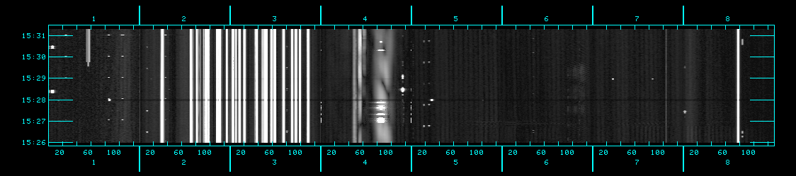
RFI is a major issue at P-band (list of P-band RFI). Of the 256 MHz frequency span that P-band observations may cover, about 30-40% may be affected by RFI. Figure 6.3.1 shows time vs. frequency of a single short baseline. The frequency range is 224-352 MHz (top) and 352-480 MHz (bottom), and the channel separation is 125 kHz. Hanning smoothing was applied to minimize Gibbs ringing.

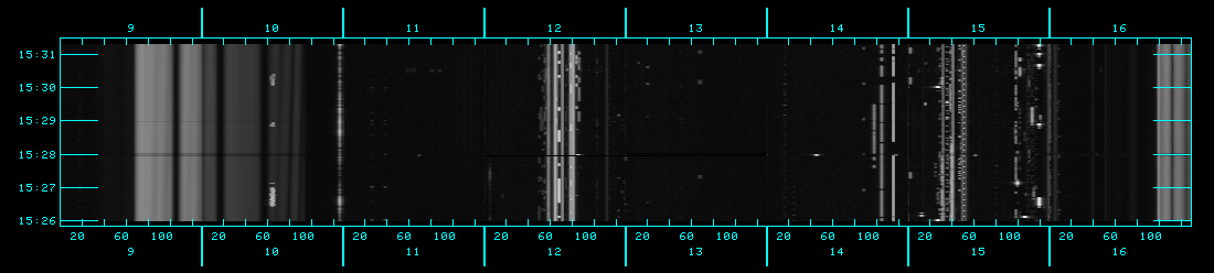Figure 6.3.1: P-band time vs. frequency for short baseline pair.

At 4-band, narrow-band RFI is generally not a major issue since most high-power analog TV channels have disappeared with only low-power TV stations transmitting below 100 MHz. Note, the presence of a self-generated RFI comb peaking at 60 MHz with a spacing of 5 MHz at antennas with old antenna control units (ACUs). This issue will improve over time with more antennas having the new generation ACUs. The comb can easily be excised, affecting only a small number of channels. Another hard to detect source of RFI, of particular concern in more compact configurations, is produced by arcing on powerlines. This produces primarily bursts of broad-band noise and can significantly affect the sensitivity of antennas near overhead powerlines and create spurious high cross-correlations. While we try to address powerline issues as they arise, the RFI environment at the VLA is still being evaluated on an ongoing basis.

Solar Activity

While observing at P-band, the following guidelines may be followed while the Sun is quiet:

In general, make sure that the Sun is more than 30° away from your sources. See the Avoiding the Sun section for more array configuration dependent details.
In D-configuration, the solar disk will likely cause a problem on the short baselines (< 100m) if the Sun is less than 90° away from the observed source.
The phases are always calibratable except during solar storms.

When the Sun is active, high solar activity results in emission that can severely affect the data to such a degree as to potentially render your observations useless. Also, such activity causes disturbing ionospheric effects. Therefore, it is imperative to avoid observing at very low frequencies at daytime (including sunrise and sunset^†) during times of high solar activity, i.e., when solar flares occur and which are more frequent during solar maximum. Solar flares with as much as a million Jy at P-band with narrow angular extents are a source of major interference. These flares are equivalent to bright, unresolved sources with time-varying flux densities that make it very difficult, if not impossible, to remove their effects. As a consequence, the resulting images will be of poor quality and low dynamic range.

Important Note: It is the responsibility of the observer to monitor if and when their sources will be too close to the Sun in addition to the activity of the Sun. If you do not want your SB(s) executed on the array due to a solar flare, which would take a few days to reach Earth after the occurrence of an eruption on the Sun, you should cancel the submission of your SB(s) through the OPT and resubmit them later. Do not rely on the operator to know about conditions relating to solar flares.

Some useful links:

Solar activity monitoring: Solar activity and general space weather can be reviewed at the NOAA site. The site provides solar activity forecasts and geophysical (geomagnetic field) activity forecasts along with GOES X-ray flux values.
Ionosphere monitoring: Global Ionospheric TEC maps or Local Ionospheric Weather from LWA.
Near real-time and archival solar activity can be seen from < 100 MHz all-sky observations by the LWA.

^†Note:The statement to avoid observing at 4/P-band at daytime (including sunrise and sunset) during times of high solar activity should not translate to checking the boxes of AVOID SUNRISE and/or AVOID SUNSET in the OPT, because these will not prohibit observing at daytime during a solar flare event. Also, these options in the OPT are not meant to address or avoid solar activity, but to avoid ionospheric phase fluctuations for low frequency observations and strong temperature gradients for high frequency observations during sunrise and sunset.

Instrument Configuration

There are three different instrument setups available to observe with the VLA at 4 and P-band:

P-band setup: Provides 16 subbands from the A0/C0 IF pair, each 16 MHz wide, to cover the frequency range 224-480 MHz, with a channel resolution of 125 KHz. The correlator integration time of this setup is 2 seconds with the 8-bit samplers.
4-band setup: Provides 8 subbands from the B0/D0 IF pair, each 4 MHz wide, to cover the frequency range 54-86 MHz, with a channel resolution of 15.6 kHz. The correlator integration time of this setup is 2 seconds with the 8-bit samplers.
4&P-band setup: This combined the two setups from above to observe 4 and P-band simultaneously.

Requantizer Setup Scans

We strongly recommend using requantizer gain level setup scans in very low frequency observations. Here we note two important sections on the use of these setup scans in 8-bit observations:

See the 8-bit General Information section under the '8/3-bit Attenuator Settings and Setup Scans' page of the VLA Observing Guide for information on how to trigger the requantizer gain setup scans while using the 8-bit samplers.
See the Special Case II in the '8/3-bit Attenuator Settings and Setup Scans' page of the VLA Observing Guide for the reasons to use the requintizer setup scans in P-band observations, and the current implementations in the Observation Preparation Tool (OPT) to utilize such scans.

Calibration

A number of calibrator observations are needed for the 4 & P-band observations. These usually include: flux density scale calibrator, complex gain (phase and amplitude gain) calibrator, and a bandpass calibrator to correct for the delays as well as the relative gains of the spectral channels even though the observations are intended for continuum science. It is recommended that the flux density calibrator be observed at least once in an observing run (a scheduling block).

Absolute Flux Density Scale

Accurate flux densities can be obtained by observing one of 3C48, 3C123, 3C138, 3C147, 3C196, 3C286, 3C295, or 3C380. P-band models are available for these sources, or at minimum a subset of, in CASA or AIPS, therefore if a given calibrator is resolved (see the VLA calibrator list), make sure to set appropriate uv ranges while executing calibration tasks. For more details on flux density calibration, see the AIPS task SETJY or the CASA task setjy.

Bandpass (and Delay)

For the VLA it is essential to calibrate the spectral response of each correlator mode used, even for purely continuum projects. For P-band observations it is necessary to use a calibrator that is > 40 Jy to properly calibrate the bandpass response, this includes continuum and spectral line projects. Some of the flux density calibrators noted above can be used for bandpass calibration at P-band. The bandpass calibrator can also be used to calibrate the delays. For calibration of 4-band data it is strictly necessary to observe a bright kJy-scale calibrator to solve for delays and bandpass. The by far single best calibrator is Cygnus A, however if observing at the galactic anticenter, depending on the array configuration and resolved structure, Taurus A or Virgo A might be suitable as well. For more details, refer to the Bandpass and Delay Calibration in the Calibration section, or the Spectral Line section.

Complex Gain (phase and amplitude gain)

Considering the large field of view of very low frequency observations, it will always be possible to self-calibrate the target phases because there will be a strong source or several strong sources within the field. It is recommended, however, to observe a complex gain calibrator (flux density > 10 Jy) with a gain cal + target + gain cal time of 30 to 60 minutes regardless of the array configuration for initial calibration and system monitoring purposes.

For more details on the above calibrators, refer to the Calibration section.

Polarization

Polarimetric observations are available for P-band only under SRO. The details for polarimetric calibration are currently being commissioned. Guidance on observation setup and calibration using AIPS is documented in EVLA Memo #207.

At 4-band due to the nature of the dipole response, the sensitivity and beam-shapes are vastly different between the two polarizations. Thus, only continuum imaging is currently commissioned below 100 MHz. It is available to perform polarimetric observations at 4-band through RSRO proposals.

Before submitting a scheduling block (SB), refer to the Presubmission Checklists:

Instrument Validation

SB Validation

Please submit any questions to the NRAO Helpdesk.