Single-band Continuum and Polarization Tutorial
In this Observation Preparation Tool (OPT) tutorial, we will create an S-band continuum polarization scheduling block (SB) to be observed in D-configuration. There are many guidelines to consider when setting up an observation.
RCT User Interface Update
The Resource Catalog Tool (RCT) had a recent UI update. This tutorial follows the steps for setting up resources using the Manual mode (aka the old RCT UI). We now have four distinct options in the RCT: Spectral Line, Frequency Sweep, Continuum, and Manual. The OPT manual has been updated to reflect the new RCT, sections of which can be found in the Resource Catalog Tool section in the OPT manual.
Guidelines for Observing S-band Continuum Polarization in D-configuration:
(For more details on the following topics, refer to the Guide to Observing with the VLA.)
- S-band Instrument Configuration: Select an NRAO default resource or create your own resource.
- Calibrators:
- complex gain (amplitude and phase)
- flux density scale
- bandpass and delay
- polarization leakage (D-term)
- polarization angle
- Calibration Strategy:
- Cycle time for appropriate phase calibration for low frequency observing in D-configuration.
- Placement of the polarization calibrators within the SB.
- LST Start Range:
- Within the SB, setup the S-band resource in one of the satellite-free zones. (Recommended, but not required.)
- Avoid elevations greater than 85°.
- Avoid elevations less than 40° (if possible) to avoid antenna shadowing. (Recommended, but not required.)
- Check to see if an antenna wrap is required.
All questions regarding this tutorial or observation setup in general, should be submitted to the NRAO Science Helpdesk under the VLA Observing department.
Accessing the OPT
To access the OPT and its suite of tools, login to the my.nrao.edu portal, or register if you have not already done so. Once you have logged in, click on the Obs Prep tab near the top and then click on the text Login to the Observation Preparation Tool (OPT) (see Figure 1).
|
|
|---|
| Figure 1: Accessing the OPT and its suite of tools. |

Instrument Configurations
Once you have logged into the OPT, click on Instrument Configurations at the top to access the Resource Catalog Tool (RCT) (see Figure 2).
|
|
|---|
| Figure 2: Accessing the Resource Catalog Tool. |

On the left-hand side within the RCT, you will see a tree titled NRAO Defaults. Open this tree by clicking on the + symbol, then select the group of defaults titled up to 2x1GHz (8bit). Figure 3 shows the first page of all NRAO Default resources where you can find your S-band resource to use (S16f5DC). By selecting the listed groups [Pointing setups, up to 4x2GHz(3bit), up to 2x1GHz(8bit)] you can narrow down the list of available default resources based upon their properties of pointing, 3-bit, or 8-bit resources.
|
|
|---|
| Figure 3: NRAO Default resources. (Click to enlarge) |

Please note that from previous NRAO Default resources there have been some changes. The first is in the description there is the "doNotChange". Default NRAO resources should not be changed by the user; if the NRAO Default does not meet your science requirements, you should create your own custom Continuum science resource, the instructions for which can be found in our documentation on Custom Type Continuum Setup.
Second, there is at the end of the resource description "dflt RFI blank". NRAO has incorporated RFI blanking to help minimize RFI. With a custom resource you can turn RFI blanking on or off. Please read our documentation on RFI blanking to learn more about this option.
For low frequency observing in D-configuration, we generally recommend a 5 second correlator integration time. The S-band resource S16f5DC (decoded in Table 1 below and seen above in Figure 3) is an appropriate choice for the observation we will be creating. Once we begin building the SB within the OPT, we will import the S16f5DC resource into the scans. Note that to see more details of the resource, you may click on the icon which looks like a blue square with a yellow bar/pencil. If needed, more information can be found in the RCT section of the OPT manual.
| S-band default resource S16f5DC | |
|---|---|
| S | frequency band |
| 16 | number of subbands (8 subbands per baseband) |
| f | full polarization (RR, LL, RL, LR) |
| 5 | correlator integration time in seconds |
| DC | suitable array configurations |
Table 1: The S-band default resource decoded.
Sources
If you have a successful proposal, about a month before the start of the proposed array configuration, your project will be imported into the OPT by NRAO staff. During this import process, a catalog of the proposed and accepted sources will be imported into the Source Catalog Tool (SCT). If you are working through this tutorial before your approved project has been made available within the OPT, this tutorial will show you how to create your own source catalog; more detail about the SCT can be found in the OPT manual.
To access the SCT, click on Sources at the top of the screen, as shown in Figure 4.
|
|
|---|
| Figure 4: Accessing the Source Catalog Tool (SCT). |
Create a New Source Catalog
To create a new source catalog, select File → Create New → Catalog (see Figure 5) then name the catalog. (Note that you may share the source catalog with others by adding them as co-I's using the Properties tab; co-I's must have a my.nrao.edu account.)
|
|
|---|
| Figure 5: Creating a new source catalog. |

Create a New Source
Once you have created the source catalog, you may add or create new sources in it. To create a new source within the catalog, select File → Create New → Source (see Figure 6).
 |
|---|
| Figure 6: Creating a new source within the catalog. |
Now you name the source and enter in the RA and Dec of the science target coordinates. For this tutorial we will be observing 3C75, a binary black hole system.
- RA: 2h 57m 42.63s
- Dec: 6d 1' 4.8"
You may copy/paste the above coordinates into the RA and Dec fields under Source Positions (see Figure 7). Be sure to hit tab or click outside of the field to allow the SCT to take the entry. Note that the SCT, RCT, and OPT do not have a save button; any changes that are made are automatically saved. Please note that if you make changes to a source position or an instrument configuration after it has been imported into a scan within the OPT, those changes will not automatically propagate throughout the scans. Instead, the resources must be re-imported into the OPT.
 |
|---|
| Figure 7: Enter source name and coordinates. |
Select the Images tab (see Figure 8) to help you determine an initial LST range of the SB. 3C75 is visible at the VLA from about 21:30-08:30 LST. This source time range is different from what we define as the LST start range of an SB. We will adjust the LST start range once we have created the SB. Note the LST start range will be restricted by other sources, i.e., the flux density calibrator.
|
|
|---|
| Figure 8: Images tab of 3C75 showing the elevation curve. |

Selecting Calibrators
Complex Gain Calibrator (Amplitude and Phase)
To search for an appropriate complex gain calibrator within the VLA calibrator database, we will use the Advanced Search feature located on the left-hand side. Select VLA from the Source Search, this enables searching the VLA calibrator database. Next, select the Cone Search parameter; enter in the RA and Dec of 3C75 (2h 57m 42.63s and 6d 1' 4.8") or select the source from the catalog you created, then widen the search radius to 15.0d (suggested maximum angle for gain calibration at low frequency), and click on the Search button. See Figure 9 for a visual guide.
With the update to 1.31 a Sky Map option has been included for the Cone Search parameters box. After entering the RA and Dec and clicking the Search button, when you click on the Sky Map icon a Sky Map will be displayed with the RA and Dec of the source in the center; this makes it easier to visualize the position of the calibrators in the sky relative to the target.
 |
|---|
| Figure 9: Advanced Search in the SCT. |
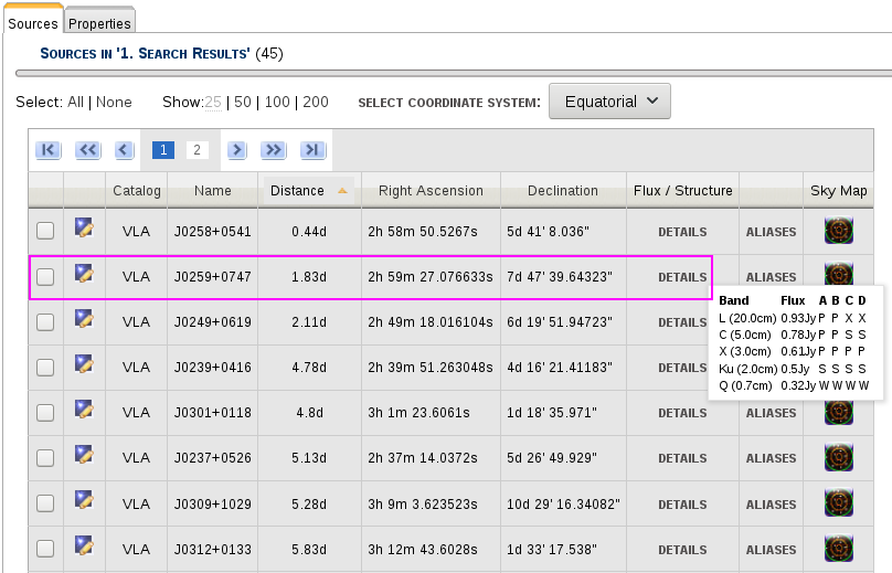
The results of the search are shown below in Figure 10. If you hover your mouse over the word Details within the SCT table, you will see the fluxes and structure codes for the known bands in the corresponding array configurations. The first calibrator in the list is not sufficient since it does not have information for the low frequencies (only Q-band). The second calibrator in the list, J0259+0747, has information for L- and C-band. Since S-band is in between these two frequency ranges, J0259+0747 can be considered and will be used in this tutorial as a complex gain calibrator. Instructions on how to choose the best complex gain calibrator can be found in the Low Frequency Strategy guide. For this particular tutorial, it is reasonable to choose J0259+0747 since it can also be used as a polarization leakage calibrator (a polarized D-term calibrator). More details regarding polarization leakage calibration will be explained later.
 |
|---|
| Figure 10: Selecting the complex gain (amplitude and phase) and polarization leakage calibrator. |
Flux Density Scale Calibrator
When selecting a flux density scale calibrator, you must choose from one of the standard 3C calibrators: 3C48, 3C286, 3C138, 3C147, and 3C295. The SCT contains a list of these 3C calibrators. Each of these 3C calibrators, except for 3C295, have models in CASA and AIPS. You can see the list by opening the tree labeled VLA (located on the left-hand side) and then select VLA Flux Cal (see Figure 11).
 |
|---|
| Figure 11: The standard VLA flux density scale calibrators, |
The structure code and the proximity of the flux density scale calibrator to the science target is not as important as when choosing the complex gain calibrator. The flux density scale calibrator should be up, have a similar LST range as the science target, and relatively close to minimize the overhead of slewing. If we do another Advanced Search centered on the science target (as explained in Figure 9 above), with a wider cone radius of 40.0d, we will find 3C48 as the closest option (32.9° from the science target). Click on the icon (blue square with a yellow bar/pencil) to the left of the source name to access the Images tab. There you will see the LST range is about 19:00-08:20, similar to 3C75 (21:30-08:30 LST).
Bandpass & Delay Calibrator
In most cases, the standard flux density scale calibrators can double as the bandpass and delay calibrator. We generally recommend using a very bright calibrator for the bandpass calibration. For this observation, we will use 3C48 as the bandpass and delay calibrator since it is very bright in the lower frequencies.
For more details regarding the complex gain, flux density scale, bandpass, and delay calibrators, refer to the Calibration section of the VLA observing guide.
Polarimetry
Since we want to image in Stokes Q and U, the instrumental polarization can be determined through observations of a bright calibrator source spread over a range in parallactic angle (> 60°). In order to determine the leakage term (i.e., the polarization impurity between the R and L polarizations, also known as the "D-term") and calibrate the absolute polarization angle, we must choose the appropriate polarization calibrators.
Polarization Leakage Calibrators
To help determine the instrumental polarization and/or to check if the instrumental polarization was properly calibrated or removed during post processing, we will use an unpolarized D-term calibrator, J2355+4950 and a polarized D-term calibrator, J0259+0747. The source J2355+4950 was chosen from Table 7.2.3 in the Polarimetry section within the VLA observing guide. We will give this source the calibrate complex gain (amplitude and phase) scan intent to ensure that, if the VLA pipeline is used to calibrate the data, its observation will be self-calibrated and can be used as an instrumental polarization calibrator if further processing is needed.
As discussed in the section above regarding the selection of the complex gain calibrator, we determined J0259+0747 is appropriate as a polarized D-term (polarization leakage calibrator) since it is known, from a recent calibrator survey for the VLA Sky Survey that included polarization information, to be 5% polarized.
For this observation, we will observe J0259+0747 for determining the instrumental polarization. An unpolarized D-term calibrator is needed only if the parallactic angle coverage is less than the recommended 60°, i.e., for short duration SBs. In this case we use the unpolarized calibrator J2355+4950 to verify the polarization leakage was correctly removed after calibration.
Polarization Angle Calibrator
3C48 will be used as the polarization angle calibrator since it has a well known polarization angle at low frequencies (S & C-band). Note its polarization fraction is only high enough to be a reliable polarization angle calibrator above 2.5 GHz.
For more details regarding the polarization calibrators, refer to the Polarimetry section of the VLA observing guide.
Observation Preparation
Now that we have chosen one of the NRAO Default S-band resources, and determined the calibrators, we can create the SB.
To access the OPT, select Observation Preparation located near the top of the screen (see Figure 12).
 |
|---|
| Figure 12: Accessing Observation Preparation. |
Create a Test Project
In order to create the SB, we will need to create a New Test Project.
Select File → Create New → Project In the pop-up box click on "TEST PROJECT" then the Add button (see Figures 13A & 13b).
if you have an accepted proposal, but it is not yet available within the OPT, you may create a Test Project to begin working on the SB(s). After the project has been made available within the OPT, you may then copy/paste the SB you've been working on into the project under the corresponding Program Block (PB).
| Figure 13A: Creating a new Project. | Figure 13B: Making a new Test Project. |
The project tree is made up of three levels:
- P: Project level contains the project code, PI, co-I's, and total allocated time.
- PB: Program Block level contains the allocated time per PB, scheduling priority, Acceptable Configurations, Linked Scheduling Blocks, list of Scheduling Blocks (SBs), and a list of Execution Blocks (once an SB has been observed).
- SB: Scheduling Block(s) contain scans with assigned sources, resources, duration (in LST), and scan intents (i.e., Setup, Observe Target, Flux Density, etc.).
Now that the Test Project has been created, you may give it a name and/or share with other co-I's, if you wish.
Edit the PB
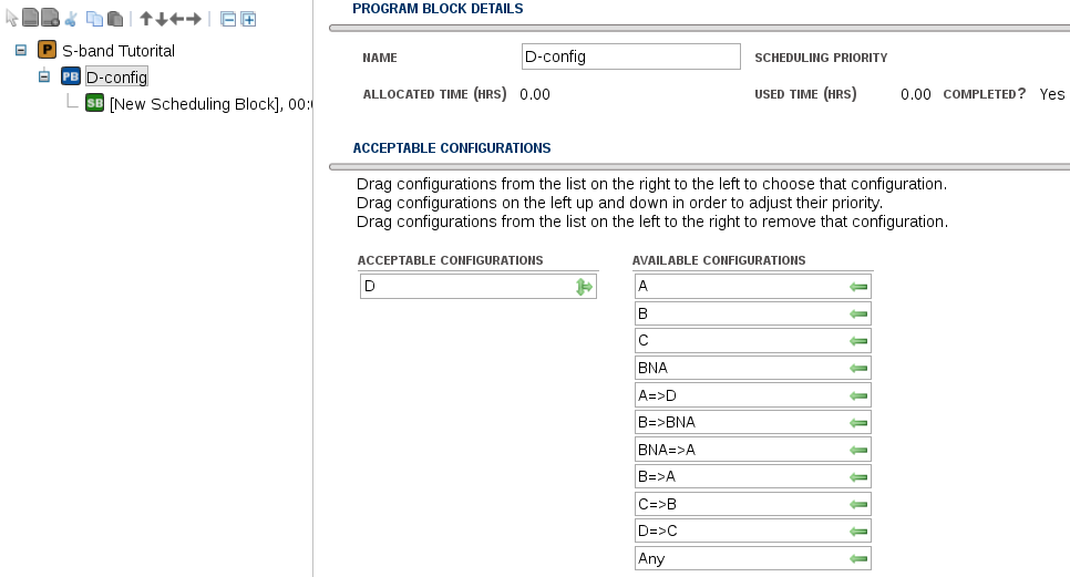
Next we will assign the PB an array configuration; this option is only available for test projects. Under the PB level of the Project, select the D under Available Configurations and drag it to the left under the Acceptable Configurations (see Figure 14). At this point you can also name the PB.
 |
|---|
| Figure 14: Assigning D to acceptable configurations and naming the PB |
Create a New SB
When creating a Project, an empty SB is automatically generated. You may use this SB or create a new SB.
To create a new SB, select File → Create New → Scheduling Block (see Figure 15).
| Figure 15: Creating a new scheduling block (SB). |
SB Information Tab
In the Information tab of the SB we can name the SB, set a preliminary LST start range of 21:30-08:30 (from the science target source, 3C75), and select the default S-band wind and Atmospheric Phase Limit (APL) constraints (see Figure 16). Recall that we will adjust the LST start range once we have finished creating the scans within the SB as, at a minimum, we would have to shorten the end time with the length of the SB.
With the update to 1.31 the Weather Constraints table has been changed to allow for alternate atmospheric phase limit values if you are planning to self-calibrate.
 |
|---|
| Figure 16: Information tab of the SB. (Click to enlarge) |
SB Setup Overview
Next we will create the scans within the SB. We should first discuss, however, the order of the scans to be created, their sources, and corresponding scan intents.
All SBs must start with at least a 1 min setup scan for all resources to be used in the observation; this will set the attenuator levels in the correlator. These levels will be set and remembered for the entire duration of the observation. Following the 1 min setup scan there should be at least a 9 min calibrator scan. This is to allow for the minimum recommended start-up for low frequency observing to be a total duration of 10 min. This start-up is to ensure plenty of slew and on source time for the first calibrator scan.
For this S-band observation, we will start with a dummy slew scan of 9 min using a different resource (e.g., C-band), followed by the 1 min setup scan for the S-band resource and then a 5 min scan on the first calibrator (in this case the flux density scale calibrator). The extra dummy slew scan is to allow the antennas to slew to one of the satellite-free zones (see Table 2) and then set the attenuator levels for the S-band resource. This 9 min duration assumes a worse-case-scenario in that the starting position for the antennas could be at its furthest from where they need to be. If this is the case, it can take up to 9 min for the antennas to slew to their destination. The AZ and EL slew rates of the antennas are 40°/min and 20°/min, respectively. Later in this tutorial we will work on adjusting the LST start range to accommodate this special start-up sequence.
| Satellite-free Zones |
|---|
| 250° < AZ < 330° and EL > 30° |
| 45° < AZ < 90° and EL < 60° |
Table 2
For more details regarding the setup scans and setting up in the satellite-free zones, refer to the 8/3-Bit Attenuator and Requantizer Gain Setup Scans in the VLA observing guide.
Table 3 below provides a basic outline of the scan duration, sources, resources, and scan intents to be used in the SB.
| Scan Duration | Source | Resource | Scan Intent(s) |
|---|---|---|---|
| 9 min | 3C48 | C-point | Setup Intent; slew to satellite-free zone |
| 1 min | 3C48 | S16f5DC | Setup Intent; set up attenuation in satellite-free zone |
| 5 min | 3C48 | S16f5DC | Calibrate Flux Density, Calibrate Bandpass, Calibrate Delay, Calibrate Polarization Angle |
| 4 min 30 sec | J2355+4950 | S16f5DC | Calibrate Complex Gain (amplitude and phase) |
| 6 min | J0259+0747 | S16f5DC | Calibrate Complex Gain (amplitude and phase), Calibrate Polarization Leakage |
| Loop x7 | |||
| 15 min | 3C75 | S16f5DC | Observe Target |
| 1 min 15 sec | J0259+0747 | S16f5DC | Calibrate Complex Gain (amplitude and phase), Calibrate Polarization Leakage |
Table 3: Basic outline of the SB.
Note that while the order of the scans is important, the order in which the scans are created is up to the observer. For example, some may prefer to create the science target scan(s) and the calibrators scans first, then create the setup scans. The OPT allows scans to be moved after creation.
Create Scans
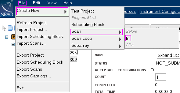
To create a new scan, select File → Create New → Scan → In (see Figure 17).
 |
|---|
| Figure 17: Creating a new scan within the SB. |
Once the scan has been created, we will change the name of the scan, import the source and resource, adjust the duration of the scan, and select the appropriate scan intents.
Source Import
To import the source, select Import (under Target Source), select VLA under Source Catalog, and you may narrow the options by selecting VLA Flux Cal under Source Group, then select either 3C48 or 0137+331=3C48, then select Change (see Figure 18).
New with 1.31 is the ability to filter your search. This is particularly handy if you are searching in the VLA catalog a source group with sources based on either RA or Dec positions. As there are many sources in the group, filtering the search by RA or Dec value can save time. In this example the VLA Flux Cal group is being accessed, which has few sources, so filtering this group isn't necessary.
 |
|---|
| Figure 18: Importing a source from the VLA calibrator catalog. |
Resource Import
To import the resource, under Hardware Setup select Import ; the default NRAO resources have been configured into four groups: All, 2x1GHz (8-bit), 4x2GH(3-bit), and Pointing setups. Since this is the dummy slew scan we will use the NRAO Default "C-point" resource. In the drop-down box for the Resource Group select Pointing setups, pick the reference pointing resource - here C-point - then select Change (see Figures 19A & 19B). Note there is nothing inherently special about choosing the C-band pointing default resource, other than it is not S-band and its default correlator integration time is 1 sec. We also could have chosen either "X-point" (both pointing resources have a 1 sec correlator integration time) or "L16f5DC" (the 5 in the name indicating a 5 sec correlator integration time).
With 1.31 you also have the ability to filter your resource by name, and/or observing band, and/or sampler. If you select a resource that does not have a sampler, e.g., L-band 3-bit, no resource will be returned. Also note that you can select multiple observing bands and samplers, e.g., C-band and X-band 3-bit and 8-bit, and a list of the resources will be returned that match these parameters. In this SB, you are selecting one of the two NRAO default reference pointing scans, of which there are only two resources, so it isn't necessary to filter the results.
 |
||
| Figure 19a: Importing a pointing resource from the NRAO Defaults. (Click to enlarge) |
Figure 19b: Selecting a pointing resource from the NRAO Defaults. |
If you haven't done so already, change the name of the scan to something that indicates what it is. This is not required, but can be helpful. The Scan Timing should be changed to 9 min to allow for plenty of slew time into one of the satellite-free zones, and change the Intents to use Setup Intent and uncheck the Observe Target intent (see Figure 20). Note that the Observe Target intent should only be used for the science target scans. An Observe Target intent selected for a setup scan or a calibrator scan will cause problems with the VLA calibration pipeline.
 |
|---|
| Figure 20: Dummy slew scan parameters. |
Copy/Paste Scans
To create all subsequent scans, we can copy/paste a scan by selecting Edit → Copy STD: <scan name> and then select Edit → Paste → Paste After STD: <scan name> (see Figures 21 and 22).
| space | ||
|---|---|---|
| Figure 21: Copy selected scan. | Figure 22: Paste after selected scan. |
S-band Setup Scan
We now make changes to this new scan for the S-band setup scan. Edit the scan Name, change the Scan Timing to 1 min (the minimum time required for setting the attenuator levels in the correlator), and import the S16f5DC resource under the Hardware Setup (see Figure 23). Notice the selected Resource Group under the NRAO Defaults is "up to 2x1GHz(8-bit)" in Figure 23. This will narrow the search for the S-band resource we decided to use earlier in this tutorial.
 |
|---|
| Figure 23: S-band setup scan. |
Calibrator Scans
Flux Density Scale, Bandpass, Delay, and Polarization Angle
Next we will copy/paste the S-band setup scan to create the first calibrator scan. Follow the same steps as seen in Figures 21 and 22 above, then change the scan Name, the Scan Timing to 5 min, and edit the scan Intents by selecting calibrate flux density scale, calibrate bandpass, then click on More >>> to select calibrate delay and calibrate polarization angle. Remember to uncheck setup intent (see Figure 24).
| Figure 24: Flux density scale, bandpass, delay, and polarization angle calibrator scan. |
Complex Gain (amplitude and phase) and Polarization Leakage
Following 3C48 will be a rather long duration scan of the secondary complex gain calibrator J2355+4950. The long duration on this calibrator scan is to ensure plenty of slew and on source time since this source is many degrees away from 3C48. The on-source time is determined by the need to obtain sufficient signal-to-noise per channel to solve for instrumental polarization. Copy/paste the flux calibrator scan, edit the scan Name, update the Target Source by importing J2355+4950, adjust the Scan Timing to 4.5 min, and select "Calibrate Complex Gain (A and P)". Remember to uncheck the other calibrator intents that were included from the copy/paste.
Next we will add another rather long scan (6 min) for the primary complex gain calibrator to ensure plenty of slew and on source time. Then we create the loop containing a science target scan and another primary complex gain calibrator scan.
Creating a Loop
To create a loop proceeding the primary complex gain calibrator, select File → Create New → Scan Loop → After (see Figure 25), then you may either copy/paste a scan or create a new scan within the loop. To copy/paste a scan into the loop, select the scan you wish to copy (use the primary complex gain calibrator), then select the loop you wish to paste the scan into, and select Edit → Paste → Paste Into Scan Name (see Figure 26). Do this last step twice so we have two scans inside the loop: one for the science target scan and one for the primary complex gain calibrator scan.
 |
space |  |
|---|---|---|
| Figure 25: Create a loop following the primary complex gain calibrator. | Figure 26: Paste the scan into the loop. |
Next we will edit the first of the two scans inside the loop to be the science target source 3C75. We can now import the source from the source catalog (see Figure 27) we made earlier in this tutorial. Then we will adjust the scan timing to 15 min, change the scan name, select Observe Target, and uncheck the calibrator intents.
 |
|---|
| Figure 27: Import science target source, 3C75. |
Next select the primary complex gain calibrator scan within the loop to adjust the scan timing to 1 min 15 sec.
Since we want the loop to be repeated 7 times, select the loop and edit the Loop Iterations field to 7. You may edit the name of the loop if you wish. Since the loop starts with the science target scan, do not select the option within the loop to bracket; if the loop were to start with the complex gain calibrator scan, then it would be appropriate to select the bracket option.
The basic layout of the SB is now complete.
LST Start Range
The next step is to adjust the LST start range to avoid the elevation limits, setup the S-band resource in one of the satellite-free zones, and avoid antenna shadowing (if possible).
To help determine an appropriate LST start range we will need to access the Reports tab of the SB. Click on the SB name and then select Reports near the top of the page (below the dark blue header). The Reports page shows the Instrument Configuration Summary, Time On Source Summary, and the Schedule Summary. We will adjust the assumed LST start to the earliest of the LST start range for 3C75 of 21:30 (click Update or hit return/enter on your keyboard) (see Figure 28). You may have noticed that, after clicking Update on the Reports page, the total duration of the SB updated (seen in the left-hand side next to the SB name). If you make a change to the length of a scan, you will need to click Update on the Reports page to force the OPT to recalculate the length of the SB.
 |
|---|
| Figure 28: Adjust the assumed LST start time on the Reports page. |
Finding the right LST start range is an iterative process by stepping through the LST start range in 5-30 min increments and then checking the Schedule Summary (bottom table on the Reports tab) to see how AZ and EL change, how slew time changes between sources/scans, and how on source time for each scan changes. We recommend at least 20 sec on source for science target and complex gain calibrator scans, and at least 40 sec on source for flux density scale, bandpass, and delay calibrator scans. Of course, more time on source may be required depending on the flux of the source and the signal to noise required for the science. When setting up your own observations, we recommend using the Exposure Calculator Tool (ECT) to help determine the appropriate time on source. This tutorial should not be used to help you determine the required time on source for your science.
Recall earlier in this tutorial the difference between the source LST range and the LST start range of an SB. If we set the assumed LST start to 08:30, you will see under the Schedule Summary table that all sources are below the VLA's horizon and the hard elevation limit of 8°. This illustrates the difference between what is meant by source LST range and LST start range.
If we set the assumed LST start to 06:00 and check the Schedule Summary, we see that all scans have an elevation greater than the recommended absolute lower elevation limit of 10°. Going through the iterative process of changing the assumed LST start and checking the Schedule Summary table, we will eventually determine the following:
- 21:30-00:55 LST is ok, however it does not setup the S-band resource within one of the satellite-free zones for the entire LST start range.
- 01:00-02:00 LST exceeds the upper elevation limit of 85°.
- 02:05-04:15 LST is the optimal start range. The S-band resource is setup in one of the satellite-free zones for the entire start range, upper and lower elevation limits are avoided, antenna shadowing is avoided, and all scans have the appropriate amount of time on source. With this LST start range, a clockwise (CW) wrap should be requested on the start-up scans (all setup scans plus the first calibrator scan).
Appendix
The SB in this tutorial was modeled after a real observation taken in D-configuration on 2018 Oct 04 UT. The data set can be downloaded from the NRAO Archive by typing in TDRW0001 into the Project (Proposal) Code field and then select TDRW0001.sb35624494.eb35628826.58395.23719237269 for download as either an SDM or an MS. The differences for the observed SB are as follows:
- Additional dummy slew scan at the start of the SB.
- A 30 sec requantizer gain setup scan for the S-band resource following the 1 min attenuator setup scan. The additional 30 sec requantizer setup scan is optional for 8-bit low frequency observations. For more details, refer to the 8/3-Bit Attenuator and Requantizer Gain Setup Scans within the VLA observing guide.
- A few extra and slightly longer scans on the primary complex gain calibrator in between two loops of the science target and the primary complex gain calibrator, causing the SB to be longer in total duration.
- LST start range used was 23:00-00:30 with a CCW antenna wrap request on the 3C48 scans. This was selected since it was in a low observing pressure range at the time of the observation. (A daily pressure histogram is posted on the Schedsoc Home Page.)
- S-band instrument configuration was modified to utilize one baseband to provide a decrease in the data rate, allowing for a smaller data set to be used for the VLA Data Reduction Workshop.
These subtle differences do not change the overall science goal of the observation, but is an example of the flexibility of setting up a low frequency observation for the VLA.
You may download and then import the xml file, S-band_tutorial.xml, into the OPT.


Connect with NRAO