test collection

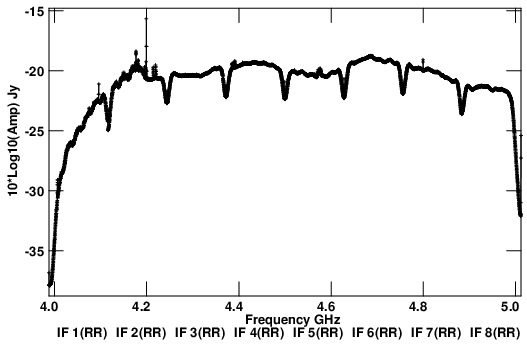
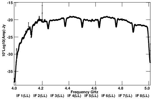
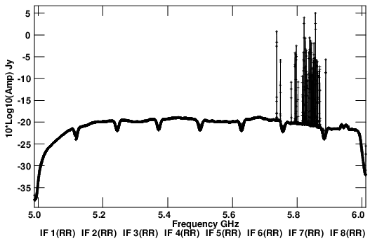
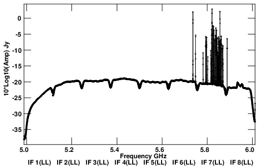
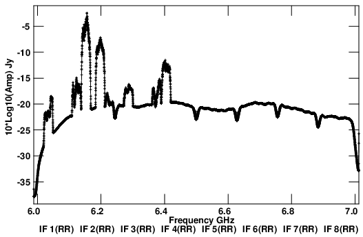
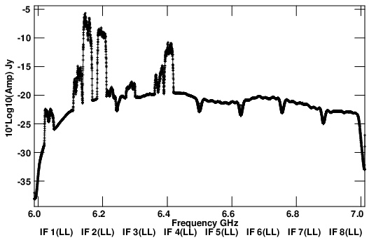
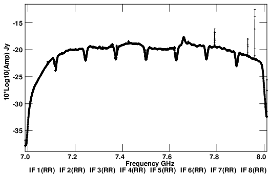
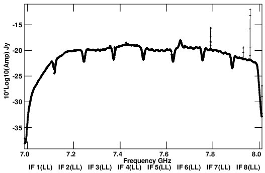
C-Band Spectra (4-8 GHz) 2025 January A-config
A listing of the various RFI in this frequency band is available here.
Also available are spectra per 128 MHz subband.
CSV files for RR and LL - 10/10
CSV files for RR and LL - 11/21
CSV files for RR and LL - 11/25
CSV files for RR and LL - 11/25
CSV files for RR and LL - 12/02
CSV files for RR and LL - 12/12
CSV files for RR and LL - 12/12
CSV files for RR and LL - 01/06
CSV files for RR and LL - 01/06
CSV files for RR and LL - 01/21
CSV files for RR and LL - 02/10
CSV files for RR and LL - 02/10
CSV files for RR and LL - 02/24
CSV files for RR and LL - 02/24
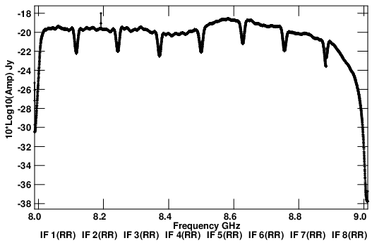
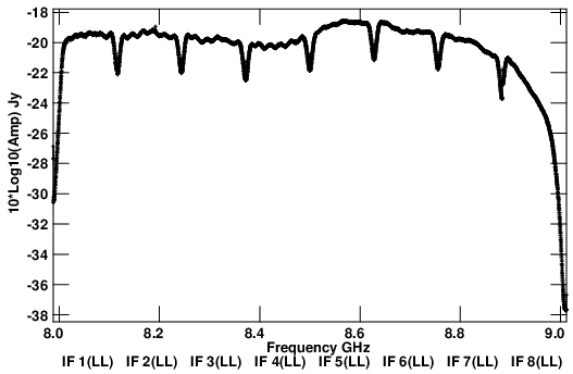
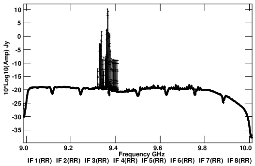
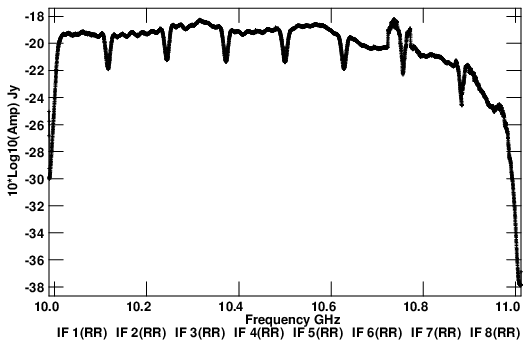
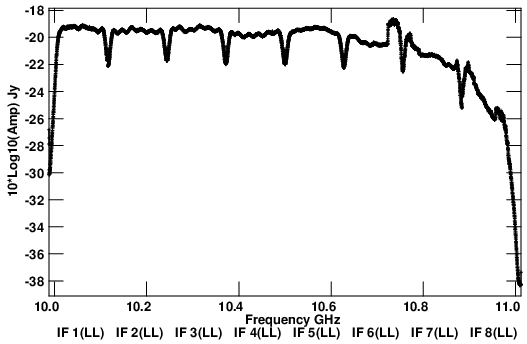
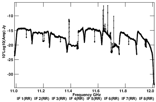
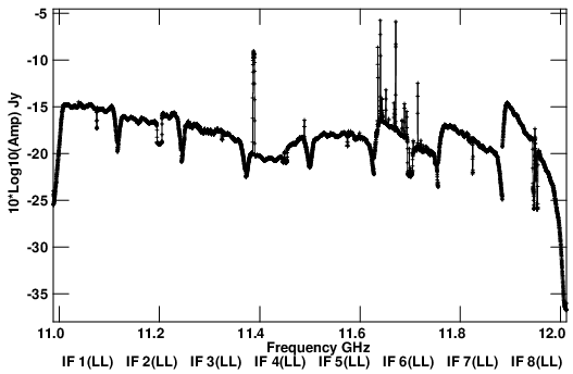
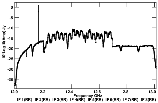
X-Band Spectra (8-12 GHz) 2025 March D-config
A listing of the various RFI in this frequency band is available here.
Also available are spectra per 128 MHz subband.
CSV files for RR and LL - 03/13
CSV files for RR and LL - 03/13
CSV files for RR and LL - 03/24
CSV files for RR and LL - 03/24
CSV files for RR and LL - 04/07
CSV files for RR and LL - 04/07
CSV files for RR and LL - 04/24
CSV files for RR and LL - 04/24
CSV files for RR and LL - 05/05
CSV files for RR and LL - 05/05

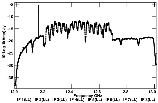
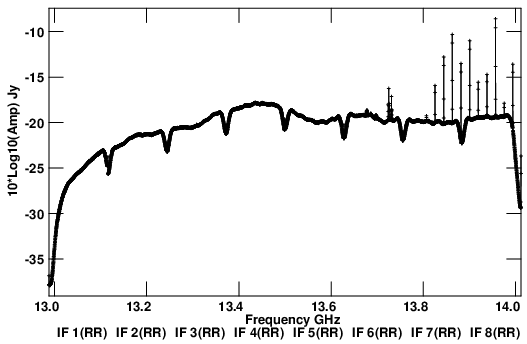
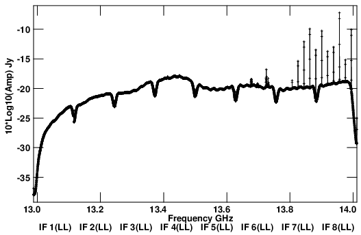
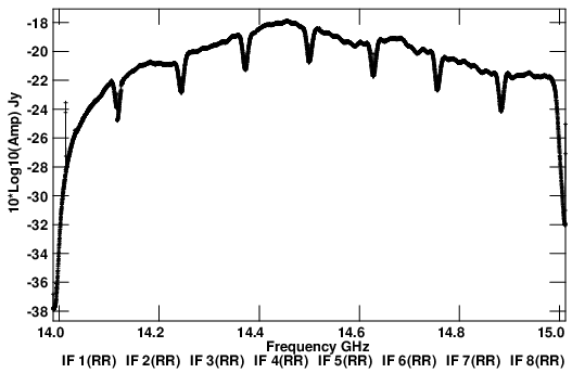
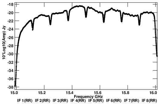
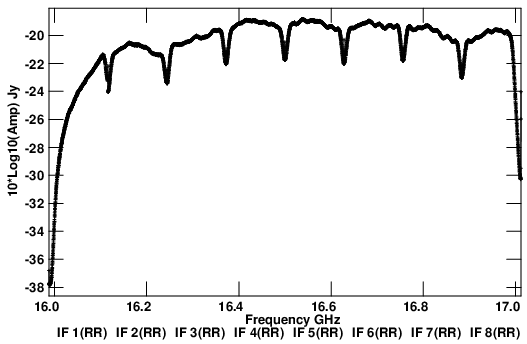
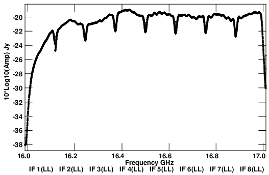
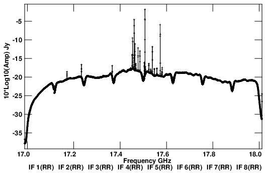
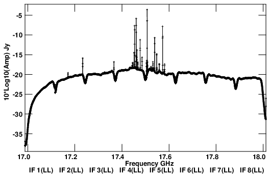
Ku-Band Spectra (12-18 GHz) 2025 March D-config
A listing of the various RFI in this frequency band is available here.
Also available are spectra per 128 MHz subband.
CSV files for RR and LL - 03/13
CSV files for RR and LL - 03/13
CSV files for RR and LL - 03/24
CSV files for RR and LL - 03/24
CSV files for RR and LL - 04/07
CSV files for RR and LL - 04/07
CSV files for RR and LL - 04/24
CSV files for RR and LL - 04/24
CSV files for RR and LL - 05/05
CSV files for RR and LL - 05/05


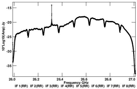
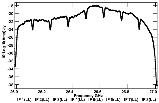
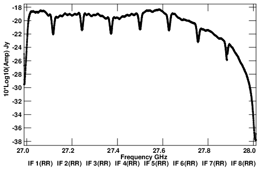
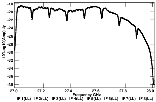
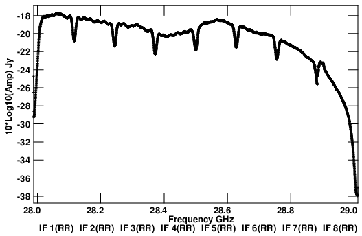
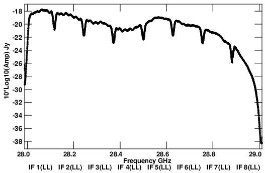
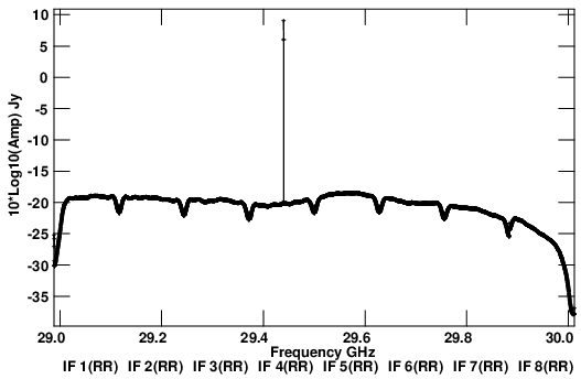
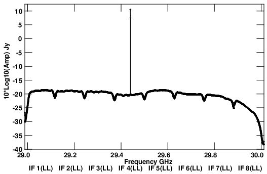
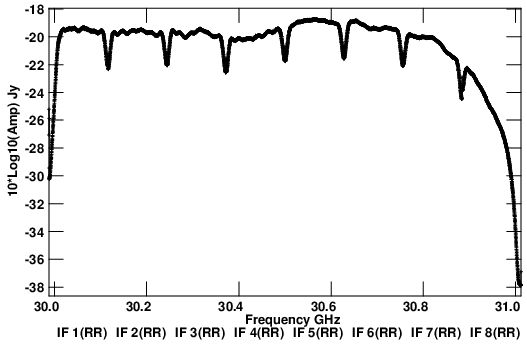
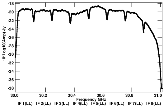
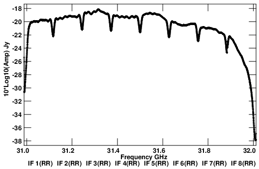
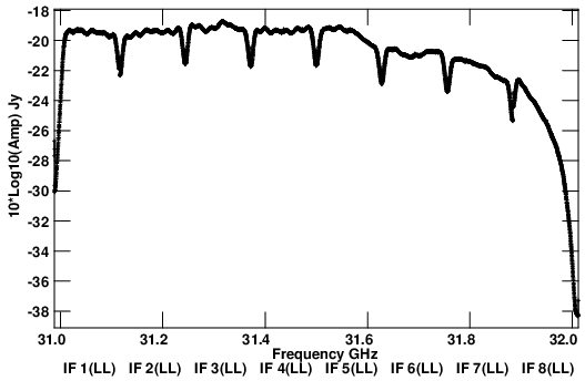
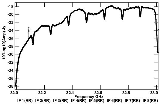
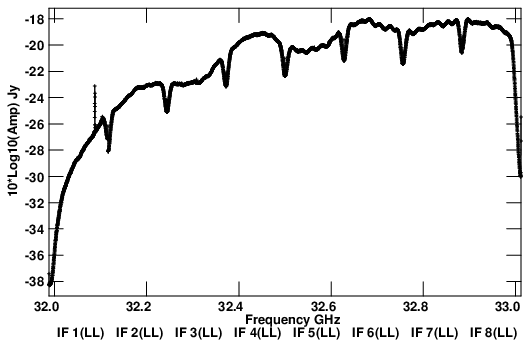
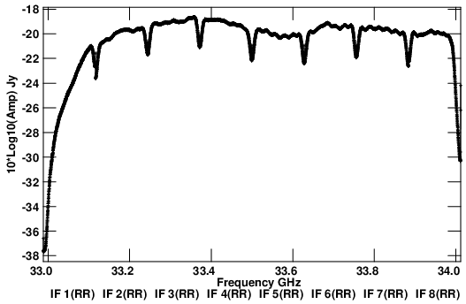
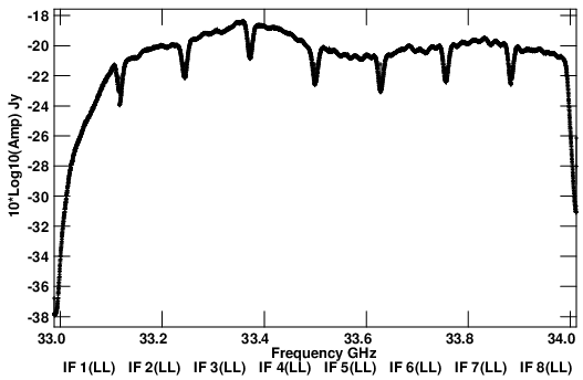
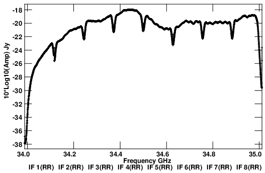
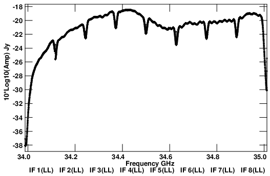
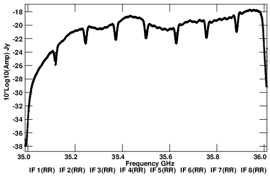
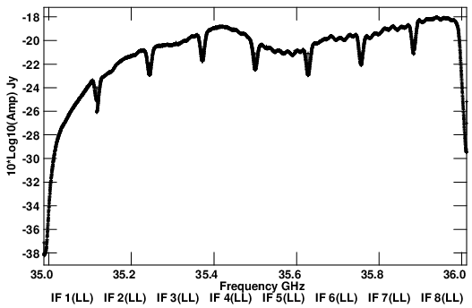
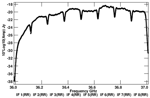
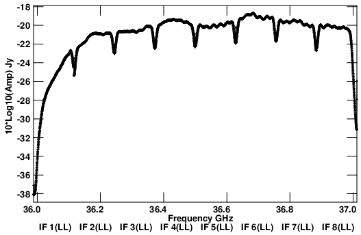
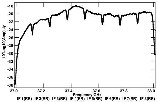
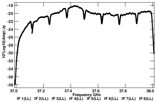
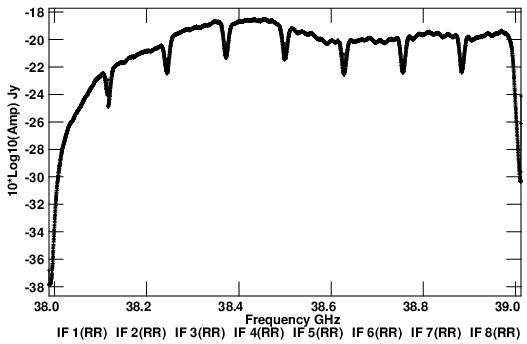
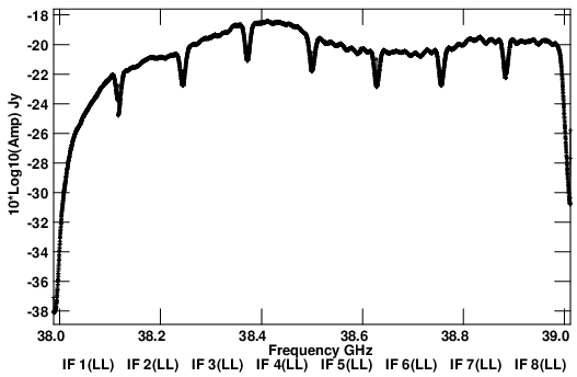
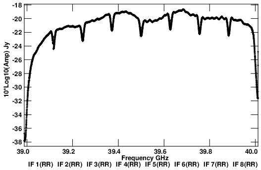
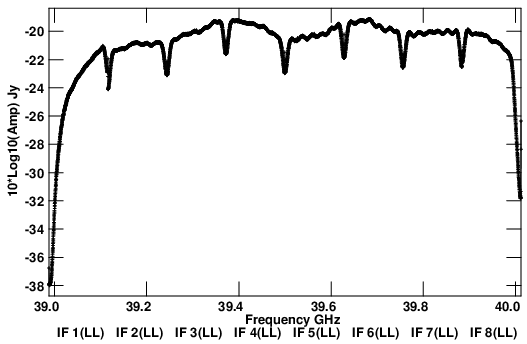
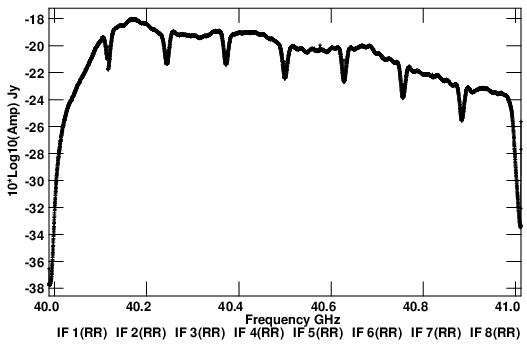
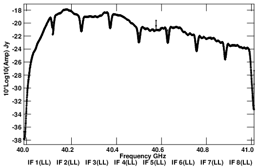
Ka-Band Spectra (26.5-40 GHz) 2025 March D-config
A listing of the various RFI in this frequency band is available here.
Also available are spectra per 128 MHz subband.
CSV files for RR and LL - 03/13
CSV files for RR and LL - 03/13
CSV files for RR and LL - 03/24
CSV files for RR and LL - 03/24
CSV files for RR and LL - 04/07
CSV files for RR and LL - 04/07
CSV files for RR and LL - 04/24
CSV files for RR and LL - 04/24
CSV files for RR and LL - 05/05
CSV files for RR and LL - 05/05
Colloquium Abstract - Harding - 2025May09
May 9, 2025
11:00am Mountain
Alice Harding (LANL)
Pulsars in the High-Energy Sky
Abstract
Of the several thousand pulsars that have been discovered by radio telescopes over the past fifty years, only a handful were known to emit gamma-ray pulsations before the launch in June, 2008 of the Fermi Gamma-Ray Space Telescope. After 17 years of operation, over 300 gamma-ray pulsars have been detected and a new population of radio-quiet pulsars has been discovered. Millisecond pulsars have been confirmed as powerful sources of gamma-ray emission, and a whole population of these objects is seen with Fermi both in the Galactic plane and in globular clusters. A gamma-ray pulsar timing array (PTA) using millisecond pulsars is now operating and may soon independently detect the gravitational wave background recently discovered by radio PTAs. Fermi has thus revolutionized the study of pulsars and allowed us to peer deeper into the inner workings of these incredibly efficient natural particle accelerators. These discoveries, together with recent progress in global simulation of pulsar magnetospheres, are changing our models of pulsar particle acceleration and high-energy as well as coherent radio emission..
Local Host: Dale Frail

")


Offered VLA Capabilities during the Next Semester
The Call for Proposals
The most recent Call for Proposals summarizes the General Observing (GO) capabilities being offered for the Karl G. Jansky Very Large Array (VLA).
In addition to these general capabilities, NRAO continues to offer shared risk observing options for those who would like to push the capabilities of the VLA beyond those offered for general use. These are the Shared Risk Observing (SRO) and Resident Shared Risk Observing (RSRO) programs.
Details about what is being offered for each program are given below. If you have any questions or problems with any link or tool, please submit a ticket through the NRAO Helpdesk.
Considering the lack of hybrid configurations after semester 2016A, guidelines on how to substitute such configurations with the use of principal array configurations are presented in the Array Configurations section of the Guide to Proposing for the VLA.
General Observing (GO) and Shared-Risk Observing (SRO)
Summary of Capabilities
As described in the Call for Proposals, the VLA offers continuous frequency coverage from 1–50 GHz in the following observing bands: 1–2 GHz (L-band); 2–4 GHz (S-band); 4–8 GHz (C-band); 8–12 GHz (X-band); 12–18 GHz (Ku-band); 18–26.5 GHz (K-band); 26.5–40 GHz (Ka-band); and 40–50 GHz (Q-band). Both single pointing and mosaics with discrete, multiple field centers will be supported under General Observing (GO). In addition to these, all VLA antennas are equipped with 224–480 MHz (P-band) and 54–86 MHz (4-band) receivers near the prime focus. Data rates of up to 60 MB/s (216 GB/hour) will be available to all users as GO, combined with correlator integration time limits per band and per configuration, as described in the Time Resolution and Data Rates section. Limitations on frequency settings and tuning ranges are described in the Frequency Bands and Tunability section.
The GO capabilities being offered are:
| Capability | Description |
| 8-bit samplers |
*Note: 4-band and dual 4/P-band observations are offered for Stokes I continuum only using standard full polarization default setups. Polarization, spectral-line, or the use of non-standard setups, should be submitted as a RSRO proposal. |
| 3-bit samplers |
|
| Mixed 3-bit and 8-bit samplers |
|
|
Subarrays |
|
| Y27 or Y1 for VLBI |
|
|
Solar observing |
|
|
On-The-Fly Mosaicking (OTF) |
|
|
Pulsar |
|
*Note: The VLA L-band (1-2 GHz) has a special signal path (the "reverse coupler" path) that allows coherent radio bursts to be observed without saturating the system, as the brightest of these solar bursts can exceed 105 solar flux units, or 109 Jy. This signal path has not yet been fully commissioned and is therefore not yet available under GO.
SRO capabilities can be set up via the Observing Preparation Tool (OPT) and run through the dynamic scheduler without intervention, but are not as well tested as GO capabilities. Data rates higher than 60 MB/s (216 GB/hour) and up to 100 MB/s (360 GB/hour) are considered SRO. A summary of the SRO capabilities being offered are:
- On-the-Fly (OTF) mosaicking for Ku-, K-, Ka-, and Q-bands (used when each pointing on the sky is on the order of several seconds or less), but not using subarrays.
- OTF observing is usually executed as linear interpolations in Equatorial Coordinates (i.e., RA/Dec). This is now also offered using interpolation linear in Galactic coordinates (l,b). Expansion in more complex patterns other than linear, such as Rosetta or Spiral patterns will remain RSRO items. Note that these must still adhere to the restrictions of the OTF mode under General Observing, i.e., using the full array below 8 GHz (up to C-band), and no subarrays.
- eLWA: Joint LWA and VLA 4-band observations using a single 8 MHz subband centered at 76 MHz, and 4-bit VDIF output. Note: During semester 2025A, the LWA is expected to be undergoing infrastructure upgrades and availability of the telescopes (LWA1 and LWA-SV) may be limited. Those interested in using this mode should contact Greg Taylor at gbtaylor@unm.edu for more details.
We expect that most SRO programs will have no or only minor problems that can be corrected quickly. If an SRO program fails, however, and it becomes clear that detailed testing with additional expertise is needed, then the project must make an experienced member from their team available to help troubleshoot the problem. In some cases, this may require the presence of that experienced member in Socorro. If adequate support from the project is not given, then the time on the telescope will be forfeited. The additional effort is to be determined based on discussions with the NRAO staff and management and the project team.
The guidelines for General and Shared Risk observing proposals, along with information about tools and other advice, can be found in the VLA Proposal Submission Guidelines.
Resident Shared Risk Observing (RSRO)
Summary of Capabilities
The VLA Resident Shared Risk Observing (RSRO) program provides users with early access to new capabilities in exchange for a period of residency in Socorro to help commission those capabilities.
RSRO proposals should be submitted using the NRAO Proposal Submission Tool in response to a regular proposal call. The proposal should include a scientific justification, as for normal proposals, which will be peer reviewed as part of NRAO's time allocation process. Selecting "VLA RSRO" from the "Observing Mode" menu on the Resources page makes an "RSRO Comments" text-entry facility available for describing the technical resources required. The text should describe the scope of the proposed RSRO work so that an accurate estimate of NRAO resources can be made by the Observatory. A description of the personnel who will be involved in the effort along with their expertise and availability should also be included in the technical justification.
We emphasize the "shared risk" nature of the RSRO program. Since observers will be attempting to use capabilities under development and in the process of being commissioned, NRAO can make no guarantee of the success of any observations made under this program, and no additional commitment is made beyond granting the hours actually assigned by the peer review process.
Proposals for any area of user interest bit offered under GO or SRO are welcome. Here, we provide some examples of capabilities that are being utilized in recent RSRO proposals.
- Correlator dump times shorter than 50 msec, including integration times as short as 5 msec for transient detection, or data rates above 100 MB/s. In order to reduce the data rate, frequency averaging in the correlator may be utilized in RSRO proposals;
- YUPPI pulsar mode combined with VLBI recording;
- Subarray observations with setups other than the default continuum setups, or observations with more than 3 subarrays.
The guidelines for Resident Shared Risk Observing proposing, along with requirements and considerations, can be found in the VLA Proposal Submission Guidelines.
Commensal Observing Systems at the VLA
There are three commensal systems on the VLA that may take data at the same time as your proposed observation. The first is the VLITE system, which will take data at P-band during regular observations that use bands other than P-band. Hence, VLITE is turned off by default during P-band or dual 4/P-band observations. The VLITE system is deployed on up to eighteen VLA antennas. Observers wishing to gain access to the commensal VLITE data taken during their VLA observations should follow the instructions on the VLITE web page for doing so. The second is the realfast system, which takes data at very fast dump rates in an effort to detect Fast Radio Bursts (FRBs). This system is fully commissioned for observing at L- through X-bands, in parallel with standard continuum correlator configurations. The third commensal system, COSMIC SETI, enables the search for extraterrestrial intelligence (SETI) using the VLA, and collects data during unconflicted PI science observations. For information about commensal observing see the Commensal Observing with NRAO Telescopes page.
To report errors or problems encountered in any link or while using any NRAO tool listed here, please submit a ticket through the NRAO Helpdesk.
Resolution
Resolution
The VLA's resolution is generally diffraction-limited, and thus is set by the array configuration and the observing frequency. Like all synthesis arrays, the VLA is sensitive only to structures on a range of angular scales between the diffraction limit (the smallest angular scale detectable) and a "Largest Angular Scale" (which depends on the fringe spacing formed by the shortest baselines in the configuration). For emission structures smaller than the diffraction limit (θ ∼ λ/Bmax), the VLA acts like a single-dish instrument—the resulting image is smoothed to the resolution of the array. For emission structures larger than the detectable range, the VLA is simply blind to the emission; this is a limitation unique to interferometers. No subsequent processing can fully recover the missing information from these large scales. It can only be obtained by observing in a more compact VLA array configuration or with data from an instrument that is sensitive to the missing angular scales, such as a large single dish or a compact array of smaller antennas.
Table 3.1.1 displays the VLA's resolution and the scale at which severe attenuation of large-scale structure occurs. This table shows the maximum and minimum antenna separations, the approximate synthesized beam size (full width at half-power; the resolution element) for the central frequency for each band, and the largest angular scale of detectable emission.
| Configuration | A | B | C | D |
|---|---|---|---|---|
| Bmax (km1) | 36.4 | 11.1 | 3.4 | 1.03 |
| Bmin (km1) | 0.68 | 0.21 | 0.0355 | 0.035 |
| Band | Synthesized Beamwidth θHPBW(arcsec)1,2,3 | |||
| 74 MHz (4) | 24 | 80 | 260 | 850 |
| 350 MHz (P) | 5.6 | 18.5 | 60 | 200 |
| 1.5 GHz (L) | 1.3 | 4.3 | 14 | 46 |
| 3.0 GHz (S) | 0.65 | 2.1 | 7.0 | 23 |
| 6.0 GHz (C) | 0.33 | 1.0 | 3.5 | 12 |
| 10 GHz (X) | 0.20 | 0.60 | 2.1 | 7.2 |
| 15 GHz (Ku) | 0.13 | 0.42 | 1.4 | 4.6 |
| 22 GHz (K) | 0.089 | 0.28 | 0.95 | 3.1 |
| 33 GHz (Ka) | 0.059 | 0.19 | 0.63 | 2.1 |
| 45 GHz (Q) | 0.043 | 0.14 | 0.47 | 1.5 |
| Band | Largest Angular Scale θLAS(arcsec)1,4 | |||
| 74 MHz (4) | 800 | 2200 | 20000 | 20000 |
| 350 MHz (P) | 155 | 515 | 4150 | 4150 |
| 1.5 GHz (L) | 36 | 120 | 970 | 970 |
| 3.0 GHz (S) | 18 | 58 | 490 | 490 |
| 6.0 GHz (C) | 8.9 | 29 | 240 | 240 |
| 10 GHz (X) | 5.3 | 17 | 145 | 145 |
| 15 GHz (Ku) | 3.6 | 12 | 97 | 97 |
| 22 GHz (K) | 2.4 | 7.9 | 66 | 66 |
| 33 GHz (Ka) | 1.6 | 5.3 | 44 | 44 |
| 45 GHz (Q) | 1.2 | 3.9 | 32 | 32 |
- These estimates of the synthesized beamwidth are for a uniformly weighted, untapered map produced from a full 12 hour synthesis observation of a source which passes near the zenith.
- Notes:
- 1. Bmax is the maximum antenna separation, Bmin is the minimum antenna separation, θHPBW is the synthesized beam width (FWHM), and θLAS is the largest angular scale structure visible to the array.
- 2. The listed resolutions are appropriate for sources with declinations between −15 and +75 degrees.
- 3. The approximate resolution for a naturally weighted map is about 1.5 times the numbers listed for θHPBW. The values for snapshots are about 1.3 times the listed values.
- 4. The largest angular scale structure is that which can be imaged reasonably well in full synthesis observations. For single snapshot observations, the quoted numbers should be divided by two.
- 5. For the C configuration, an antenna from the middle of the north arm is moved to the central pad N1. This results in improved imaging for extended objects, but may slightly degrade snapshot performance. Note that although the minimum spacing is the same as in D configuration, the surface brightness sensitivity and image fidelity to extended structure is considerably inferior to that of the D configuration.
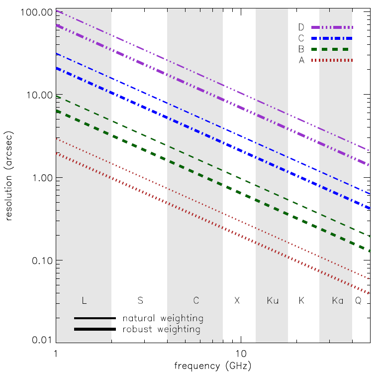
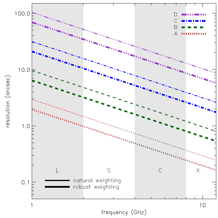
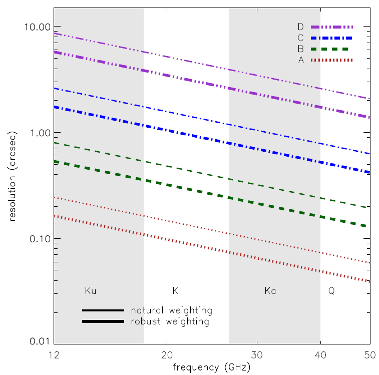
The following figure is a graphical representation of the synthesized beamwidths for natural and robust weighting for the four main array configurations between 1 and 50 GHz. Also available are synthesized beamwidth figures for the low frequency (1–12 GHz) and the high frequency (12–50 GHz) receiver bands.
(click image to enlarge)
Sensitivity
Sensitivity
The theoretical thermal noise expected for an image using natural weighting of the visibility data is given by:
| \[\Delta I_m = \frac{SEFD}{\eta_{\rm c}\sqrt{n_{\rm pol}N(N-1)t_{\rm int}\Delta\nu}}\] | (eq. 1) |
where:
- - SEFD is the system equivalent flux density (Jy), defined as the flux density of a radio source that doubles the system temperature. Lower values of the SEFD indicate more sensitive performance. For the VLA's 25–meter paraboloids, the SEFD is given by the equation SEFD = 5.62Tsys/ηA, where Tsys is the total system temperature (receiver plus antenna plus sky), and ηA is the antenna aperture efficiency in the given band.
- - ηc is the correlator efficiency (~0.93 with the use of the 8-bit samplers).
- - npol is the number of polarization products included in the image; npol = 2 for images in Stokes I, Q, U, or V, and npol = 1 for images in RCP or LCP.
- - N is the number of antennas.
- - tint is the total on-source integration time in seconds.
- - Δν is the bandwidth in Hz.
Figure 3.2.1 shows the SEFDs as a function of frequency used in the VLA exposure calculator for those Cassegrain bands currently installed on VLA antennas, and include the contribution to Tsys from atmospheric emission at the zenith. Figure 3.2.2 shows the SEFDs as a function of frequency for the P-band; these measurements are based on imaging of a field far from the galactic plane. Table 3.2.1 gives the SEFD at some fiducial VLA frequencies.
 |
 |
Figure 3.2.1: SEFD used in the Exposure Calculator for the VLA. Left: The system equivalent flux density as a function of frequency for the L, S, C and X-band receivers. Right: The system equivalent flux density as a function of frequency for the Ku, K, Ka, and Q-band receivers. SEFDs at Ku, K, Ka, and Q bands include contributions from Earth's atmosphere and were determined under good conditions.
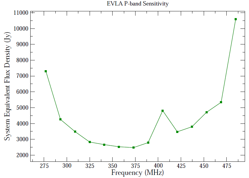
Figure 3.2.2: The SEFD used in the VLA Exposure Calculator as a function of frequency for the P-band receiver
Note that the theoretical rms noise calculated using equation 1 is the best limit possible. There are several factors that will tend to increase the noise compared with theoretical:
- For the more commonly used robust weighting scheme, intermediate between pure natural and pure uniform weightings (available in the AIPS task IMAGR and CASA task clean), typical parameters will result in the sensitivity being a factor of about 1.2 worse than the listed values.
- Confusion. There are two types of confusion: (i) that due to confusing sources within the synthesized beam, which affects low resolution observations the most. Table 3.2.1 shows the confusion noise in D configuration assuming robust weighting (see Condon et al. 2012, ApJ, 758), which should be added in quadrature to the thermal noise in estimating expected sensitivities. The confusion limits in C configuration are approximately a factor of 10 less than those in Table 3.2.1; (ii) confusion from the sidelobes of uncleaned sources lying outside the image, often from sources in the sidelobes of the primary beam. This confusion primarily affects low frequency observations.
- Weather. The sky and ground temperature contributions to the total system temperature increase with decreasing elevation. This effect is very strong at high frequencies, but is relatively unimportant at the other bands. The extra noise comes directly from atmospheric emission: primarily from water vapor at K-band, and from water vapor and the broad wings of the strong 60 GHz O2 transitions at Q-band.
- Losses from the 3-bit samplers. The VLA's 3-bit samplers incur an additional 10–15% loss in sensitivity above that expected—i.e., the efficiency factor ηc = 0.78 to 0.83.
| Frequency | SEFD (Jy) |
RMS confusion level |
||
|---|---|---|---|---|
| 0.39 GHz (P) | 2790 | 5330 | ||
| 1.5 GHz (L) | 420 | 74 | ||
| 3.0 GHz (S) | 370 | 12 | ||
| 6.0 GHz (C) | 310 | 2 | ||
| 10.0 GHz (X) | 250 | negligible | ||
| 15 GHz (Ku) | 320 | negligible | ||
| 20 GHz (K) | 500 | negligible | ||
| 33 GHz (Ka) | 600 | negligible | ||
| 45 GHz (Q) | 1300 | negligible |
In general, the zenith atmospheric opacity to microwave radiation is very low: typically less than 0.01 at L, C, and X-bands; 0.05 to 0.2 at K-band; and 0.05 to 0.1 at the lower half of Q-band, rising to 0.3 by 49 GHz. The opacity at K-band displays strong variations with time of day and season, primarily due to the 22 GHz water vapor line. Observing conditions are best at night and in the winter. Q-band opacity, dominated by atmospheric O2, is considerably less variable.
Observers should remember that clouds, especially clouds with large water droplets (thunderstorms), can add appreciable noise to the system temperature. Significant increases in system temperature can, in the worst conditions, be seen at frequencies as low as 5 GHz.
Tipping scans—which are currently unavailable but will be implemented at some time in the future—can be used for deriving the zenith opacity during an observation. In general, tipping scans should only be needed if the calibrator used to set the flux density scale is observed at a significantly different elevation than the range of elevations over which the complex gain calibrator (amplitude and phase) and target source are observed.
When the flux density calibrator observations are within the elevation range spanned by the science observing, elevation dependent effects (including both atmospheric opacity and antenna gain dependencies) can be accounted for by fitting an elevation-dependent gain term. See the following items:
- Antenna elevation-dependent gains. The antenna figure degrades at low elevations, leading to diminished forward gain at the shorter wavelengths. The gain-elevation effect is negligible at frequencies below 8 GHz. The antenna gains can be determined by direct measurement of the relative system gain using the AIPS task ELINT on data from a strong calibrator which has been observed over a wide range of elevation. If this is not possible, care should be taken to observe a primary flux calibrator at the same elevation as the target.
Both CASA and AIPS allow the application of elevation-dependent gains and an estimated opacity generated from ground-based weather through the CASA tasks gencal and plotweather, and AIPS task INDXR.
- Pointing. The SEFD quoted above assumes good pointing. Under calm, nighttime conditions, the antenna blind pointing is about 10 arcsec rms. The pointing accuracy in daytime can be much worse—occasionally exceeding 1 arcminte due to the effects of solar heating of the antenna structures. Moderate winds have a very strong effect on both pointing and antenna figure. The maximum wind speed recommended for high frequency observing is 11 mph (5 m/s). Wind speeds near the stow limit 45 mph (20 m/s) will have a similar negative effect at 8 and 15 GHz.
To achieve increased pointing accuracy, referenced pointing is recommended where a nearby calibrator is observed in interferometric pointing mode every hour or so. The local pointing corrections measured can then be applied to subsequent target observations. This reduces rms pointing errors to as little as 2–3 arcseconds (but more typically 5–7 arcseconds) if the reference source is within about 15 degrees in azimuth and elevation of the target source and the source elevation is less than 70 degrees. At source elevations greater than 80 degrees (zenith angle < 10 degrees), source tracking becomes difficult; it is recommended to avoid such source elevations during the observation preparation setup.
Use of referenced pointing is highly recommended for all Ku, K, Ka, and Q-band observations, and for lower frequency observations of objects whose total extent is a significant fraction of the antenna primary beam. It is usually recommended that the referenced pointing measurement be made at 8 GHz (X-band), regardless of what band your target observing is at, since X-band is the most sensitive and the closest calibrator is likely to be weak. Proximity of the reference calibrator to the target source is of paramount importance; ideally the pointing sources should precede the target by 20 or 30 minutes in Right Ascension (RA). The calibrator should have at least 0.3 Jy flux density at X-band and be unresolved on all baselines to ensure an accurate solution.
To aid VLA proposers there is an online guide to the exposure calculator; the exposure calculator provides a graphical user interface to these equations.
Special caveats apply for P-band (230–470 MHz) observing. The SEFD's in Figure 3.2.2 or that listed in table 3.1.2 are from an observation taken far from the Galactic plane, where the sky brightness is about 30K. At P-band, Galactic synchrotron emission is very bright in directions near the Galactic plane. The system temperature increase due to Galactic emission will degrade sensitivity by factors of two to three for observations in the plane, and by a factor of five or more at or near the Galactic center. Additionally, the antenna efficiency (currently about 0.31 for 300 MHz) will decline with both increasing and decreasing frequencies from the center of P-band.
The beam-averaged brightness temperature measured by a given array depends on the synthesized beam, and is related to the flux density per beam by:
| \[T_{\rm b} = \frac{S \lambda^2}{2k\Omega} = F \cdot S\] | (eq. 2) |
where Tb is the brightness temperature (Kelvins) and Ω is the beam solid angle. For natural weighting (where the angular size of the approximately Gaussian beam is ∼1.5λ/Bmax), and S in mJy per beam, the parameter F depends on the synthesized beam, therefore on the array configuration, and has the approximate value of F = 190, 18, 1.7, 0.16 for A, B, C, and D configurations, respectively. The brightness temperature sensitivity can be obtained by substituting the rms noise, ΔIm, for S. Note that Equation 2 is a beam-averaged surface brightness; if a source size can be measured, then the source size and integrated flux density should be used in Equation 2 and the appropriate value of F calculated. In general, the surface brightness sensitivity is also a function of the source structure and how much emission may be filtered out due to the sampling of the interferometer. A more detailed description of the relation between flux density and surface brightness is given in Chapter 6 of Reference 1, listed in Documentation.
For observers interested in HI in galaxies, a number of interest is the sensitivity of the observation to the HI mass. This is given by van Gorkom et al. (1986; AJ, 91, 791):
| \[M_{\rm HI} = 2.36 \times 10^5 D^2 \sum S \Delta V ~~~~M_\odot\] | (eq. 3) |
where D is the distance to the galaxy in Mpc, and SΔV is the HI line area in units of Jy km/s.
VLA Frequency Bands and Tunability
-
- 1. Listed here are the nominal band edges. For all bands, the receivers can be tuned to frequencies outside this range, but at the cost of diminished performance. Contact the NRAO Helpdesk for further information.
- 2. The 4-band system is currently under development. The default frequency range maximizes sensitivity of the system and provides a nominal bandwidth of 12 MHz and a channel resolution of 64 kHz.
- 3. The default setup for P-band will provide 16 subbands from the A0/C0 IF pair, each 16 MHz wide, to cover the frequency range 224–480 MHz. The channel resolution is 125 kHz.
- 4. The default frequency setup for L-band comprises two 512 MHz IF pairs (each comprising 8 contiguous subbands of 64 MHz) to cover the entire 1–2 GHz of the L-band receiver.
Tuning Restrictions
In general, for all frequency bands except Ka, if the total span of the two independent IF pairs of the 8-bit system (defined as the frequency difference between the lower edge of one IF pair and the upper edge of the other) is less than 8.0 GHz, there are no restrictions on the frequency placements of the two IF pairs. For K, Ka, and Q-bands—the only bands where a span greater than 8 GHz is possible—there are special rules:
- At Ka-band, the low frequency edge of the A0/C0 IF pair must be greater than 32.0 GHz. There is no restriction on the B0/D0 frequency, unless the B0/D0 band overlaps the A0/C0 band when the latter is tuned at or near the 32.0 GHz limit. In this case, the Observation Preparation Tool (OPT) may not allow the requested frequency setups. Users wanting to use such a frequency setup are encouraged to contact the NRAO Helpdesk for possible tuning options.
- At K and Q-bands, if the frequency span is greater than 8.0 GHz, the B0/D0 frequency must be lower than the A0/C0 frequency.
For the 3-bit system, the maximum frequency span permitted for the A1/C1 and A2/C2 IF pairs is about 5000 MHz. The same restriction applies to B1/D1 and B2/D2. The tuning restrictions given above for the separation and location of the 8-bit pairs A0/C0 and B0/D0 also apply to the 3-bit pairs, with A0/C0 replaced by A1/C1 and A2/C2, and B0/D0 replaced by B1/D1 and B2/D2.
VLA Samplers
The VLA is equipped with two different types of samplers, 8-bit with 1GHz bandwidth, and 3-bit with 2GHz bandwidth. The choice depends on your science goals and on technicalities described below.
The 8-bit Set consists of four 8-bit samplers running at 2.048 GSamp/sec. The four samplers are arranged in two pairs, each pair providing 1024 MHz bandwidth in both polarizations. The two pairs are denoted A0/C0 and B0/D0. Taken together, the four samplers offer a maximum of 2048 MHz coverage with full polarization. The frequency spans sampled by the two pairs need not be adjacent. Some restrictions apply, depending on band, as described in the section on Frequency Bands and Tunability.
The 3-bit Set consists of eight 3-bit samplers running at 4.096 GSamp/sec. The eight samplers are arranged as four pairs, each pair providing 2048 MHz bandwidth in both polarizations. Two of these pairs, denoted A1/C1 and A2/C2 cannot span more than 5000 MHz (lower edge of one to the higher edge of the other). The same limitation applies to the second pair, denoted B1/D1 and B2/D2. The tuning restrictions are described in the section on Frequency Bands and Tunability. Taken together, the eight 3-bit samplers offer a maximum of 8192 MHz coverage with full polarization.
Which set to use?
- S, L, and 4/P-band observations, whether line or continuum, should use the 8-bit sampler set.
- C and X-band continuum observations should use 3-bit samplers in order to exploit the full 4 GHz bandwidth: in spite of the 15% reduction in sensitivity that comes with 3-bit (at equal bandwidth to the 8-bit samplers—see below for details) and the reduced effective bandwidth after removing RFI, this still provides superior overall sensitivity. For more details we refer to EVLA memo 166.
- Note: C-band is impacted by strong RFI caused by microwave links near 6 GHz in the A and B configurations. As a result, 3-bit data obtained with the standard setup are corrupted. We advise observers to use mixed 3-bit and 8-bit samplers. For more details, refer to the VLA Observing Guide.
- Ku, K, Ka, and Q-band continuum observations should use the 3-bit samplers for maximum bandwidth.
- Wide-band spectral line searches requiring more than 2 GHz span should use the 3-bit samplers.
- Spectral-line observations which fit within two, possibly disjoint, 1 GHz bands should use the 8-bit set.
- Simultaneous continuum and high resolution spectral line observation can use mixed 3-bit and 8-bit samplers. The 3-bit samplers in this case will be set up to deliver the continuum data, while the 8-bit samplers will be for the spectral line data. This mix mode can be used in C-band and higher.
Major Characteristics of each Set
The 8-bit samplers are warranted for observations at 4/P, L, and S-bands. The full analog bandwidth from the receivers fits within the 2048 MHz span covered by the samplers.
For the 3-bit samplers, users need to be aware of the following issues:
- Sensitivity: compared to the 8-bit system, the sensitivity of the 3-bit samplers is worse by ~15% (at equal bandwidth). Alternatively, a given continuum noise level requiring on-source integration time T with the 8-bit (two bands of 1GHz), requires 0.33T with the 3-bit (4 bands of 2GHz, assuming the bandwidth is available from the front end).
- Resonances: each of the eight 3-bit samplers on an antenna has a resonance about 3 MHz wide. Each resonance is independent of all others, so there is no correlated signal between antennas. The resonance degrades the spectrum in its narrow frequency range, but has little effect on continuum observing. Bandpass solutions will be affected, but can be interpolated over. Spectral-line calibration and images at the affected frequencies will show significant loss in sensitivity. The resonances are easily seen in autocorrelation spectra, and it is recommended that users, especially spectral-line users, utilize these to locate the compromised frequencies.
- Amplitude Calibration: The traditional method for both 8- and 3-bit systems is to observe a flux-density calibrator, use self-cal to determine the antenna amplitude calibration factors (gains), and transfer the gains to the phase calibrator and target. For 3-bit samplers this procedure gives results good to 5% between elevations of 20–70 degrees. (Expect worse at the upper edge of Q-band and/or during bad weather.) The switched power data can be used to correct for system gain variations and works well for the 8-bit samplers. For 3-bit samplers, the Pdif depends on the Psum, i.e., Pdif is non-linear and its application will bias the resulting visibilities by 5–10%. The origin of this effect is understood, but we have not yet determined how best to compensate for it. Because of this, we do not recommend use of the Psum and Pdif data to calibrate visibilities from the 3-bit samplers. We do, however, recommend that the requantizer gains in the switched power data be applied to remove gain changes. For more information about the switched power, Psum, and Pdif, see EVLA memo 145.
Setting up the 8-bit or 3-bit Samplers
Either set requires an initial scan for each individual LO (frequency) tuning, during which power levels are optimized.
For the 8-bit system, a dummy scan of 1 minute duration is sufficient for each tuning. This is usually done while the antennas are slewing at the start of an observing file, as the pointing direction of the antennas is not critical.
For the 3-bit system, the requirements are more demanding, see the section on 3-bit setup within the Guide to Observing with the VLA. The minimum setup time is 1 minute for each tuning to adjust the power levels and bandpass slopes across the 2GHz samplers. These values are retained and applied if the tuning is re-encountered in the same observation. Additionally, every time the LO setup is changed—whether or not it is new (e.g., changing from 8-bit X-band reference pointing back to target)—a scan of 30 seconds is needed to reset the subband gains (requantizers) in the correlator. For better amplitude calibration at high frequencies, the 3-bit initial setup should be near the elevation of the target, so do it after the first 8-bit setup described above. For 3-bit observing without 8-bit (e.g., C or X-band without reference pointing), the power variation with elevation is small, so the 3-bit setup can be done at any elevation.
For settings that use a mix of 3-bit and 8-bit samplers, the guidelines to set up the 3-bit samplers should be followed.
Other issues
The overhead for setup of 3-bit samplers can eat into observing time, especially for projects with many different LO settings, and/or sources all over the sky accompanied by band change, reference pointing, and requantizer reset for each direction. The impact is most severe for short scheduling blocks.
Polarization testing conducted so far indicates no degradation of performance by using the 3-bit samplers.
Time Resolution and Data Rates
The default integration times for the various array configurations and frequency bands are as follows:
| Configurations | Observing Bands |
Default integration time |
|---|---|---|
| A, B, C, D | 4 P | 2 seconds |
| A | L S C X Ku K Ka Q | 2 seconds |
| B | L S C X Ku K Ka Q | 3 seconds |
| C, D | X Ku K Ka Q | 3 seconds |
| C, D | L S C | 5 seconds |
Observations with the 3-bit (wideband) samplers, when applicable, should use these integration times. Observations with the 8-bit samplers may use shorter integration times, but these must be requested and justified explicitly in the proposal, and obey the following restrictions:
| Proposal type |
Minimum integration time |
Maximum data rate |
|---|---|---|
| General Observing (GO) | 50 msec | up to 60 MB/s (216 GB/hr) |
| Shared Risk Observing (SRO) | 50 msec | > 60 MB/s (216 GB/hour) and up to 100 MB/s (360 GB/hour) |
| Resident Shared Risk Observing (RSRO) | < 50 msec | > 100 MB/s (360 GB/hr) |
Note that integration times as short as 5 msec and data rates as high as 300 MB/s can be supported for some observing, though any such observing is considered Resident Shared Risk Observing. For these short integration times and high data rates there will be limits on bandwidth and/or number of antennas involved in the observation. Those desiring to utilize such short integration times and high data rates should consult with NRAO staff.
The maximum recommended integration time for any VLA observing is 10 seconds.
Observers should bear in mind the data rate of the VLA when planning their observations. For Nant antennas and integration time Δt, the data rate† is:
| Data rate | ~ 45 MB/sec × (Nchpol/16384) × Nant × (Nant − 1)/(27×26) / (Δt/1 sec) |
| ~ 160 GB/hr × (Nchpol/16384) x Nant × (Nant − 1)/(27×26) / (Δt/1 sec) | |
| ~ 3.7 TB/day × (Nchpol/16384) × Nant × (Nant − 1)/(27×26) / (Δt/1 sec) |
Here Nchpol is the sum over all subbands of spectral channels times polarization products:
| Nchpol = Σi Nchan,i × Npolprod,i |
where Nchan,i is the number of spectral channels in subband i, and Npolprod,i is the number of polarization products for subband i (1 for single polarization [RR or LL], 2 for dual polarization [RR and LL], 4 for full polarization products [RR, RL, LR, LL]). This formula, combined with the maximum data rates given above, imply that observations using the maximum number of channels currently available (16384) will be limited to minimum integration times of ~2 seconds for standard observations, and 0.8 seconds for shared risk observations.
We note that frequency averaging in the correlator will reduce the total number of channels. Therefore, the data rate and the data volume will be reduced by the same channel averaging factor. See the Chromatic Aberration section for more details on the frequency averaging in the correlator and to assess its impact on your science.
These data rates are challenging for transfer and analysis. Data may be downloaded via ftp over the Internet. For users whose science permits, the Archive Access Tool allows some level of frequency averaging in order to decrease data set sizes before ftp; note that the full spectral resolution will be retained in the NRAO archive for all observations.
†Note: The data rate formula given above does not account for the auto-correlations delivered by WIDAR. Precise data rate values can be obtained through the use of the Resource Catalog Tool for proposing (RCT-proposing).
Radio Frequency Interference
The very wide bandwidths of the VLA mean that radio frequency interference (RFI) will be present in a far larger fraction of current observations than in observations made with the old systems. Considerable effort has gone into making the VLA's electronics as linear as possible, so that the effects of any RFI will remain limited to the actual frequencies at which the RFI exists. Non-linear effects, such as receiver saturation, should occur only for those very unlikely, and usually very brief, times when the emitter is within the antenna primary beam.
RFI is primarily a problem within the low frequency (C, S, L, and the low-band system) bands, and is most serious in the D configuration. With increasing frequency and increasing resolution comes an increasing fringe rate, which is often very effective in reducing interference to tolerable levels.
The bands within the tuning range of the VLA which are protected for radio astronomy are: 73.0-74.6 MHz, 322.0-328.6 MHz, 1400–1427 MHz, 1660.6–1670.0 MHz, 2690–2700 MHz, 4990–5000 MHz, 10.68–10.7 GHz, 15.35–15.4 GHz, 22.21–22.5 GHz, 23.6–24.0 GHz, 31.3–31.8 GHz, and 42.5–43.5 GHz. No significant external interference should occur within these bands.
VLA staff periodically observes the entire radio spectrum with the VLA, from 1.0 through 50.0 GHz with 125 kHz channel resolution, to monitor the ever-changing RFI spectrum. Users concerned about the precise frequencies of strong RFI, and the likelihood of being affected, are encouraged to peruse these plots. To access these plots, or for more information on RFI, including the impact of satellite transmissions, please see the RFI section in the Guide to Observing with the VLA.
Subarrays
The continuum subarray option offers two 1 GHz baseband pairs with the 8-bit samplers in up to 3 subarrays or four 2 GHz baseband pairs with the 3-bit samplers, with the same spectral channel and polarization product options as are available for wideband observing. The setup for each subarray is completely independent in terms of observing frequency, polarization products, and integration times.
When using three subarrays, there are some restrictions on the number of antennas in each subarray. The Baseline Board in the correlator treats each set of 4 antennas independently, using a separate column of correlator chips. With 7 such columns, the correlator can handle up to 7×4 = 28 antennas. The correlator configuration software requires that a given column not be split across subarrays. For instance, one cannot observe with 9 antennas in each of 3 subarrays, because 9 antennas requires three columns (two with 4 antennas each, and one with 1 antenna); three subarrays of 9 antennas each would require 3×3 = 9 columns, two more than are actually available. Splitting the array into 11, 8, and 8 antennas is allowed.
For more information on subarrays, please see the Subarrays section in the Guide to Observing with the VLA.
Positional Accuracy & Astrometry
The position of a target can be determined to a small fraction of the synthesized beam, limited by atmospheric phase stability, the proximity of an astrometric calibrator, the calibrator-source cycle time, and the SNR on target.
In preparation for observing, the a priori position must be known to within the antenna primary beam, except perhaps for mosaicking observations. In the special case of using the phased VLA as a VLBI element, the a priori position must be accurate to within the synthesized beam of the array.
In post-processing, target positions are typically determined from an image made after phase calibration, i.e., correcting the antenna and atmospheric phases as determined on the reference source. The accuracy of the calibration determines the accuracy of the positions in the image. Note that phase self-calibration imposes the assumed position of the model, i.e., makes the position indeterminate. Therefore, an absolute position cannot be determined after self-calibration, but relative positions between features within a self-calibrated image are valid.
It may help to think of astrometry as two methods, narrow-field and wide-field.
Narrow-field astrometry
In narrow-field astrometry, the target is close to the phase tracking center and the antennas nod every few minutes between the target and a calibrator. If no special calibration provisions are taken, under typical conditions, an astrometric accuracy of ~10% of the synthesized beam FWHM can often be obtained. For example, an observation in Ka-band (~33 GHz) in A-configuration might reach an astrometric accuracy of ~10 milliarcseconds (mas). When care is taken (special calibrations and ideal observing conditions), the accuracy can approach 1–2% of the synthesized beam, with a floor of ~2 mas. If such accuracies are needed, we strongly recommend obtaining advice from VLA staff in setting up the observations.
Astrometric calibrators are marked J2000 A in the VLA calibrator list, and have a positional accuracy of ~2 mas. Other catalogs from the USNO and the VLBA are also useful, but offsets may exist between the VLA and VLBA centroids arising from extended structure in the particular source and the different resolutions of the arrays.
For studies of proper motion and parallax, the absolute accuracy of a calibrator may be less important than its stability over time. Close, or in-beam calibrators with poor a priori positions, can be used and tied to the ICRF reference frame in the same or separate observations.
Phase stability can be assessed in real time from the Atmospheric Phase Interferometer (API) at the VLA site, which uses observations of a geostationary satellite at ~12 GHz. Dynamic scheduling uses the API data to run a project under suitable conditions specified by the user. VLBI projects using the phased VLA will typically be fixed date and not dynamically scheduled.
Wide-field astrometry
Wide-field astrometry is used to determine the positions of targets within the primary beam, referenced to a calibrator within the beam or close by. In addition to the previous effects, there are distortions as a function of position in the field, from small errors in the Earth Orientation Parameters (EOP) used at correlation time, differential aberration, and phase gradients across the primary beam. With no special effort, the errors build up to roughly one synthesized beam at a separation of ~104 beams from the phase tracking center. Not all these errors are fully understood, and accurate recovery of positions over the full primary beam in the wide-band, wide-field case is a research area. These effects are handled somewhat differently in the post-processing packages. Check with VLA staff for more details via the NRAO Helpdesk.
Calibrating the Flux Density Scale
Normal calibration of the flux density scale for VLA observations is effected by including a scan on a source of presumed known flux density in each Scheduling Block (SB). Using that known flux density source, the flux density of the complex gain calibrator(s) can be determined and then transferred to your target source(s). Historically, 3C48 and 3C286 have been the standard sources for which NRAO has assumed flux densities are known as a function of frequency, and which have been recommended as flux density scale calibrator sources for the VLA. Restrictions on baseline length as a function of VLA configuration and observing band were supplied which, if followed, allowed relatively accurate flux density scale calibration. We have recently improved the ability to calibrate the flux density scale by providing sky brightness models for these sources in CASA and AIPS, which loosens the restrictions on configurations and bands. We have also added the sources 3C138* and 3C147 to the list of calibrators that have models. However, 3C48, 3C138*, and 3C147 have spectral flux densities that vary with time (3C286, along with 3C295 and 3C196, are constant), so some care should be taken if the most accurate flux density scale calibration is desired.
Note: While accurate models are available in both AIPS and CASA for various frequency bands for the calibrators 3C286, 3C48, 3C147, and 3C138*, neither 3C295 nor 3C196 has such models in CASA. Therefore, the VLA CASA calibration pipeline will fail if these two calibrators are used. Furthermore, 3C295 and 3C196 may not be suitable for all VLA configurations and frequencies even if one chooses to not use the pipeline.
A single observation of a few minutes of one of the above-mentioned flux density scale calibrators will suffice for most observers. If possible, the flux density scale calibrator should be observed at a time when it is nearly at the same elevation as the complex gain calibrator, especially for the highest four bands (Ku-, K-, Ka-, and Q-band). This is not always possible because of timing and geometry of sources, and that it is not typically known when an SB will be executed (so elevations versus time are uncertain). Flux density scale calibration accuracy in this case should be of order 10% at 4- and P-bands, 5% at L- through Ku-bands, and 10-15% for the three higher bands. If more accuracy is needed, a more careful strategy should be adopted, potentially using multiple flux density scale calibrators. The fundamental accuracy of the scale is ~5% at 4- and P-bands, 3% at L- through Ku-bands, increasing to 5% at Q-band. See Perley and Butler (2017) for more details on how the spectral flux densities of 3C48, 3C138*, 3C147, and 3C286 (and many other sources) have been determined across the frequency range from 50 MHz to 50 GHz and how they vary versus time, along with information on the fundamental accuracy of the flux density scale when using these sources.
If less accuracy is needed in the flux density scale calibration, an observation of one of these standard sources need not necessarily be included in an SB. As an example, for a short triggered observation where a simple detection is desired, the time spent slewing back and forth to the flux density scale calibrator can make the SB significantly longer than it could otherwise be. In this scenario, the switched power measurement can be used to calibrate the flux density scale; see EVLA Memo 120 for some background. This technique, which should only be used with the 8-bit samplers, is not a standard path of calibration, but it is possible. The flux density scale accuracy in this case is ~10% for L- through Ku-bands, increasing to ~20% at Q-band; not nearly as good as using the "standard" method of flux density scale calibration, but it may be sufficient for some observers.
For reference, the polynomial expression for the spectral flux density for 3C286 determined in Perley and Butler (2017) is: \[\log(S) = 1.2481 - 0.4507 \log(f) - 0.1798 \log^2(f) + 0.0357 \log^3(f)\] where S is the flux density in Jy, and f is the frequency in GHz.
The tables below show flux densities determined using the polynomial coefficients for a few sources at a single frequency within each of the VLA bands.
| Source | 75 MHz | 350 MHz | 1500 MHz | 3000 MHz | 6000 MHz | 10000 MHz | 15000 MHz | 22000 MHz | 33000 MHz | 45000 MHz |
|---|---|---|---|---|---|---|---|---|---|---|
| 3C48 = J0137+3309 | 72.8 | 42.2 | 15.4 | 8.44 | 4.42 | 2.68 | 1.79 | 1.22 | 0.815 | 0.601 |
| 3C138* = J0521+1638 | 26.5 | 16.1 | 8.25 | 5.44 | 3.39 | 2.33 | 1.72 | 1.28 | 0.949 | 0.761 |
| 3C147 = J0542+4951 | 58.0 | 52.3 | 21.0 | 12.0 | 6.45 | 3.99 | 2.73 | 1.93 | 1.39 | 1.13 |
| 3C196 = J0813+4813 | 129 | 44.4 | 13.6 | 6.98 | 3.38 | 1.91 | 1.20 | 0.763 | 0.473 | 0.329 |
| 3C286 = J1331+3030 | 30.0 | 25.9 | 14.6 | 9.91 | 6.39 | 4.50 | 3.37 | 2.54 | 1.88 | 1.49 |
| 3C295 = J1411+5212 | 124 | 58.4 | 21.2 | 11.0 | 5.06 | 2.70 | 1.60 | 0.970 | 0.571 | 0.385 |
| Source | 328 MHz | 1465 MHz | 2565 MHz | 4885 MHz | 6680 MHz | 11320 MHz | 16564 MHz | 25564 MHz | 32064 MHz | 48064 MHz |
|---|---|---|---|---|---|---|---|---|---|---|
| 3C48 = J0137+3309 | 43.9 | 15.6 | 9.82 | 5.48 | 4.12 | 2.56 | 1.86 | 1.33 | 1.11 | 0.816 |
| 3C138* = J0521+1638 | 15.9 | 8.26 | 6.00 | 4.00 | 3.23 | 2.24 | 1.69 | 1.25 | 1.06 | 0.821 |
| 3C147 = J0542+4951 | 53.9 | 21.4 | 13.8 | 7.88 | 5.91 | 3.67 | 2.61 | 1.82 | 1.53 | 1.14 |
| 3C196 = J0813+4813 | 46.5 | 13.8 | 8.14 | 4.22 | 3.00 | 1.67 | 1.08 | 0.656 | 0.508 | 0.313 |
| 3C286 = J1331+3030 | 25.8 | 14.6 | 10.9 | 7.33 | 5.97 | 4.12 | 3.15 | 2.30 | 1.92 | 1.44 |
| 3C295 = J1411+5212 | 61.1 | 21.6 | 12.8 | 6.42 | 4.45 | 2.33 | 1.43 | 0.819 | 0.596 | 0.405 |
We refer the reader to the VLA Observing Guide for the practical considerations (e.g., observing frequency and array configuration, as well as post processing) regarding the choice of the flux density scale calibrator in their scheduling blocks.
* The flux density scale calibrator 3C138 is currently undergoing a flare. As of January 2025, the change in flux density is greater than 10% at all frequencies greater than 4 GHz (i.e., C-band). At present, the magnitude of the flare is approximately a factor of 2 at K-band, 3 at Ka-band, and 4 at Q-band. Monthly monitoring observations are available for investigators that require an accurate flux density scale when using 3C138. These observations are publicly available in the archive under the project code TCAL0009. A table of scaling factors per band per month from February 2021 onward has been provided.
Complex Gain Calibration
General Guidelines for Complex Gain Calibration
Adequate complex gain calibration (tracking amplitude and phase fluctuations as a function of time) is a complicated function of source-calibrator separation, frequency, array scale (configuration), and weather. Since what defines adequate for some experiments is completely inadequate for others, it is difficult to define simple guidelines to ensure adequate phase calibration. However, some general statements remain valid most of the time. These are given below.
- Under decent conditions with no thunderstorms or ionospheric storms, tropospheric effects dominate at frequencies higher than about 4 GHz; ionospheric effects dominate at frequencies lower than about 4 GHz.
- Atmospheric (troposphere and ionosphere) effects are nearly always unimportant in the C and D configurations at L and S-bands, and in the D configuration at X and C-bands. For these cases, calibration need only be done to track instrumental changes—three or four times per hour is usually sufficient for tracking the system gains.
- If your target object has sufficient flux density to permit phase self-calibration, there is no need to calibrate more than a couple of times per hour at low frequencies or 15 minutes at high frequencies in order to track pointing or other effects that might influence the amplitude scale. The enhanced sensitivity of the VLA guarantees, for full-band continuum observations, that every field will have enough background sources to enable phase self-calibration at L and S-bands. At higher frequencies, the background sky is not sufficient, and only the flux of the target source itself will be available.
- In principle, the smaller the source-calibrator angular separation, the better (even if the closer calibrator is weaker). However, the final choice will depend on the observing frequency. If deciding between a nearby calibrator with an S code in the calibrator database, and a more distant calibrator with a P code, for low frequencies (L-band and below) the nearby calibrator is usually the better choice (low frequency strategy). For higher frequencies it is advisable to use the further away but higher quality P-code calibrator (high frequency strategy). A detailed description of calibrator codes is available in the calibrator list.
- Phase stability often deteriorates dramatically after about 10AM due to small-scale convective cells set up by solar heating, even in clear and calm conditions, especially in the summer. Observers should consider a more rapid calibration cycle for observations between this time and a couple of hours after sundown.
- At high frequencies, and longer configurations, rapid switching between the source and nearby calibrator is needed to track tropospheric phase fluctuations if the target cannot be self-calibrated. See Rapid Phase Calibration and the Atmospheric Phase Interferometer (API) (below).
Rapid Phase Calibration and the Atmospheric Phase Interferometer
Polarization
For projects requiring imaging in Stokes Q and U, the instrumental polarization should be determined through observations of a bright calibrator source spread over a range in parallactic angle or a single observation of an unpolarized source. The complex gain calibrator chosen for the observations can also double as a polarization calibrator, provided it is at a declination where it moves through enough parallactic angle during the observation (roughly Dec 15–50 degrees during a several hour track).
The minimum condition that will enable accurate polarization calibration from a polarized source, in particular with unknown polarization, is three observations of a bright source spanning at least 60 degrees in parallactic angle (schedule four scans, if possible, in case one is lost); if at all possible, it is strongly recommended that five or more observations covering 100 degrees (or more) of parallactic angle in roughly uniform steps be run. If a bright, unpolarized, unresolved source is available, and known to have very low polarization, then a single scan will suffice to determine the leakage terms. The accuracy of polarization calibration is generally better than 0.5% for small objects as compared to the antenna beam size. At least one observation of 3C286 or 3C138 is required to fix the absolute position angle of polarized emission; 3C48 can be used at frequencies of ~3 GHz and higher, or 3C147 at frequencies over ~10 GHz. Note that 3C48 and 3C138 are variable—the polarization properties are known to be changing significantly over time, most notably at the higher frequencies (for details see Perley and Butler (2013b)).
More information on polarization calibration strategy can be found in the Polarimetry section in the Guide to Observing with the VLA.
VLBI Observations
The VLA can participate in VLBI observations with the VLBA. This is possible by either using the VLA as a phased array (Y27) or using one of its dishes (single dish: Y1). We note that currently P-band cannot be phased. For more details see the VLBI at the VLA documentation. In phased array mode, the program TelCal derives the antenna-based delay and phase corrections needed for antenna phasing in real time. This correction is applied to the antenna signals before they are summed, requantized to 2-bits, and recorded in VDIF format on the Mark5C disk at the VLA site. The disk(s) are then transported to Socorro, NM and correlated on the DiFX correlator with other VLBI stations which participated in the observation.
Standard VLA data, i.e., correlations between VLA antennas, are also archived in the NRAO science data archive. By default, a maximum of 512 MHz dual polarization is phased/recorded and sent to the archive. This leaves a large portion of the possible VLA bandwidth unused (up to 2 or 8 GHz total depending on sampler choice). Increasing the bandwidth to the maximum that the VLA can provide has obvious benefits for most continuum observations. Pulsar gating can be performed commensally with the phased VLA, avoiding the need for extra single dish observations. Line VLBI observations that run through the WIDAR correlator currently produce each requested VLBI subband bandwidth divided into full polarization products with 64 frequency channels, regardless of the requested spectral resolution obtained in the VLBI correlation. By adding unused baseline boards to the VLBI-specified line subbands, a closer match in spectral resolution can be offered for the standalone VLA data. If you think your science could benefit from these capabilities, please review our documentation on VLBI at the VLA or contact the helpdesk for further guidance.
Snapshots
The two-dimensional geometry of the VLA allows a snapshot mode whereby short observations can be used to image relatively bright, unconfused sources. This mode is ideal for survey work where the sensitivity requirements are modest.
Single snapshots with good phase stability of strong sources should give dynamic ranges of a few hundred. Note that because the snapshot synthesized beam contains high sidelobes, the effects of background confusing sources are much worse than for full syntheses, especially at 20 cm and longer wavelengths in the D configuration. For instance, at 20 cm, a single snapshot will give a limiting noise of about 0.2 mJy. This level can be reduced by taking multiple snapshots separated by at least one hour. The deconvolution of the data is necessary to remove the effects of background sources. Before considering snapshot observations at 20 cm, users should first determine if the goals desired can be achieved with the existing Faint Images of the Radio Sky at Twenty-centimeters survey (FIRST, http://sundog.stsci.edu/top.html) (B configuration) or the NRAO VLA Sky Survey (NVSS, http://www.cv.nrao.edu/nvss/) (D configuration, all-sky).


Connect with NRAO