Multi-band, Multi-spectral Line, and Continuum Tutorial

Observation Preparation Tool Tutorial

This document describes how to create VLA observing scripts using the Observation Preparation Tool (OPT) and its associated suite of tools: the Source Catalog Tool (SCT) and the Resource Catalog Tool (RCT). We will use an example source (science target) and resource (instrument configuration) to show how to design an observing script, more commonly called a Scheduling Block (SB), using the OPT. After following this tutorial, you should be able to create an SB appropriate for your science goals.

Note that this tutorial does not replace or substitute for the more complete content that can be found in the official, full content OPT Manual, in the Guide to Observing with the VLA, or in the VLA Observational Status Summary (etc.).

RCT User Interface Update

The Resource Catalog Tool (RCT) had a recent UI update. This tutorial follows the steps for setting up resources using the Manual mode (aka the old RCT UI). We now have four distinct options in the RCT: Spectral Line, Frequency Sweep, Continuum, and Manual. Refer to the Spectral Line section of the OPT manual for the new RCT guidelines.

The Science Case

Before starting anything it is good to review what was written in the proposal for which this observing time was granted. Apart from the actual time and configuration allocation, here may also be useful information in the comments or technical review of the disposition letter. Here we will use the numbers given below and assume they were extracted from a hypothetical proposal; how they were derived and argued for are not relevant for this tutorial.

We want to observe a planetary nebula, NGC 2371, for thermal and maser lines and possible associated stellar continuum. In the hypothetical proposal we argued we need D-configuration to potentially detect extended ammonia hyperfine emission, NH₃(1,1), NH₃(2,2), and the potentially point-like water and hydroxyl masers. The rest frequencies and spectral resolution we are trying to capture are listed in the table below, as well as the anticipated time on source to achieve our RMS noise and brightness temperature. The time allocation is 2.5 hours and all velocities are assumed in the LSR Radio frame.

Science Target from Hypothetical Proposal
	NGC 2371	Notes
Coordinates (J2000)	07h 25m 34.68s, +29d 29' 26.4"	planetary nebula
Velocity	21 km/s	LSR/Radio frame
LST range	02:16 to 18:51	lower elevation limit of 25 degrees

Instrument Configurations (resources)
	Line Frequency (MHz)	Coverage (km/s)	Resolution (km/s)	Notes
L-band				about 15 min on-source in L-band
OH 1612	1612.2310	100	0.2
OH 1665	1665.4018	100	0.2
OH 1667	1667.3590	100	0.2
OH 1720	1720.5300	100	0.2
K-band				about 1h45m on source in K-band
H₂O	22235.1	100	0.1
NH₃(1,1)	23694.5 (23692.9-23696.1)	100	2.3	hyperfine lines span 3.2 MHz
NH₃(2,2)	23722.6 (23720.5-23724.7)	100	2.3	hyperfine lines span 4.2 MHz
continuum	K-band	—	—

Other line frequencies for the VLA can be found in the line list in the OPT manual.

The Approach

To observe this experiment, the SB must contain the details of the science target source(s), calibrator(s), and resource(s). For calibrators and continuum resources, the SCT and RCT provide standard catalogs with calibrator positions and default instrument configurations, respectively. In general, the science target and spectral line setup should be provided by the observer before the SB can be created. The basic steps are as follows:

Supply the science target source coordinates to the SCT and determine appropriate calibrators;
Create the spectral line resource in the RCT or any other personalized (continuum) resource;
Create an SB in the OPT by combining sources and resources into an ordered scan list.

Steps 1 and 2 can be done in reverse order. For continuum observations, step 2 can be skipped if an NRAO default resource is used, and step 1 can be skipped if the science target source(s) has already been imported and the calibrators have been determined. In this tutorial, however, each step will be shown to explain the components of the SCT, RCT, and OPT. During this process, remember to create unique names for catalogs, sources and resources.

Define Source Coordinates in the SCT

If the proposal was submitted to NRAO using the Proposal Submission Tool (PST), the coordinates entered in the PST will transfer to the SCT about a month before the first eligible array configuration (an email notification will be sent to the PI and co-I's). If the proposal was allocated time through another Time Allocation Committee (TAC) (e.g., a NASA panel), this transfer of source(s) to the SCT will not occur. In any case, log into the OPT with your my.nrao.edu login and navigate to the SCT by selecting the Obs Prep tab, then click on Login to the Observation Preparation Tool, and then click on Sources located in the dark blue navigation bar at the top (see Figure 1).


Figure 1: The OPT navigation bar.

There are three ways to define sources in the SCT:

Direct transfer from the PST, done by NRAO staff;
Upload of a text file (e.g., the same that was uploaded/exported from the PST), or;
Manual creation of each source in the SCT.

If there is a source catalog labeled with a proposal code in the left-hand side below the VLA source catalog, it is likely that the source positions were transferred from the PST to the SCT. Click on the source catalog name to view the list of sources in the catalog and check that the positions entered in the PST conform to the accuracy needed. This is important, particularly if the PST only contains regions (e.g., for mozaics) or approximate coordinates.

If there is no catalog for the project, if the catalog is empty, or if the source coordinates are not accurate enough, then the source coordinates need to be entered or updated by the user.

If you have the source list that was uploaded to the PST for your proposal at hand, you can upload this list (with or without updates, using the same PST format) by selecting from the menu File → Import. You can add a line with the anticipated catalog name if it is the first line of the file and that line starts with an asterisk (or modify the New Catalog later in the properties tab). Example PST format files are given in the source list explanation in the OPT manual text-file section.

If needed, and for the purpose of learning the components of the SCT, create a new catalog by selecting from the menu File → Create New → Catalog (see Figure 2).


Figure 2: Create a new source catalog.

Give the new catalog an appropriate name in the Properties tab, e.g., "18A: NGC2371"; then select the Sources tab (see Figure 3).


Figure 3: Selecting the Sources tab under the new source catalog.

Next, create a new source by selecting from the menu File → Create New → Source (see Figure 4).


Figure 4: Creating a new source.

Provide a name and the coordinates that represent the field center (see Figure 5). When done, return to the catalog by selecting its name (on the left) or select "Return to <catalog name>" (located above the tabs). Repeat these steps for other sources.


Figure 5: Enter source information. (Click to enlarge.)

When looking at the catalog listing, click on the blue icon on the left of a row to enter the source properties to make additional edits such as updating the PST-transferred position, or click on the right-most black icon (see Figure 6) to see which calibrators are nearby in the bulls-eye tool (opens a new browser tab) and remember any suitable ones for your target positions (see Figure 7).


Figure 6: Sources in catalog information. (Click to enlarge.)


Figure 7: Bulls-eye view of calibrators surrounding your source. Number 1 is calibrator J0714+3534, 6 deg from the science target source, while number 2 is the location of the Sun at the LST date and time this screen capture was created. Note: if you have a source in your catalog and it is within the area of sky of the sky map, it will appear yellow. (Click to enlarge.)

While it is useful to copy your calibrators to the catalog, this is not required as they are already defined in the VLA calibrator list. As an example of how this is done, use the Advanced search in the upper left-hand side of the SCT (see Figure 8).


Figure 8: Advanced Search. (Click to enlarge)

Select the VLA catalog and any other catalog you want to search.
Click the Cone Search box to activate the parameters field.Type in the coordinates of your target (which do not have to be very accurate, e.g., 7h 25m and 29d 30'), and a radius of the cone to search.
Click on the Search button.

Note that besides the Search button there are two other options that can be performed, Save and Download, that will appear after the Search has been executed. After performing a search, you can either select calibrators (see Figure 10) and save them to a new catalog which is automatically generated and placed in the left-hand tree; or you can select the Download button which will create a text file of your selected calibrator(s) and download the file to your local computer's Download folder.

The sources that match the selection criteria, here within 10 degrees of the position, are listed at the bottom and sorted by increasing distance from the entered position. Hover over the Details field of each source to judge the flux and structure for use as a phase calibrator for your project (see Figure 9).


Figure 9: The source details pop up when hovering over the "Details" field of the source in the table; J0741+3112 will be the complex gain calibrator for this observation at both L and K-bands.

If none of the sources match your requirements, use a larger search radius. Otherwise either list the source name for future use, or click the checkbox in front of the calibrator you want to use and select from the menu Edit → Copy → Sources (see Figure 10) to copy the source.


Figure 10: Using Edit → Copy → Sources from the general calibrator list after a search. (Click to enlarge)

Select the complex gain calibrator(s) by checking the box(es)
In the Menu select Edit
From the drop down menu select Copy
From the fly out menu select Sources

Now, paste it into your project catalog (click the project catalog and then select from the menu Edit → Paste → Sources (see Figure 11). You can do this as many times as you want. You may want to also include your flux density and bandpass/delay calibrators, and if applicable also any polarization and reference pointing calibrators.


Figure 11: Using Edit → Paste → Sources to the project's source catalog. (Click to enlarge)

From the Menu select File
From the drop down menu select Paste
From the fly out menu select Sources

If you have selected coordinates near the science target (NGC 2371), you will find that source J0741+3112 is bright (>1 Jy/beam at any frequency) and has useful calibrator properties (code P and S) for the low and high frequency ranges in compact array configurations. Because of its simple structure, we can use this calibrator as a phase (complex gain) calibrator for both the L- and K-band observations. Because the calibrator is bright and approximately flat spectrum, we may also use it as a delay and bandpass calibrator, especially if it is brighter than our flux density calibrator. For high-frequency observations we need a pointing calibrator, bright and point-like in X-band, and this calibrator can be used for that as well.

For a flux density calibrator, simply go to the Flux Cal group in the VLA list (located on the left) (see Figure 12 step 1). Note, 1411+522=3C295 should only be used at low frequencies (P- and L-band) in the compact array configurations (C- and D-configuration). Here we can use 0137+331=3C48 at the beginning of the SB or 1331+305=3C286 at the end; both are selected (Figure 12 step 2). You then perform a copy of the sources (Figure 12 steps 3, 4, and 5). Repeat Figure 11 steps 1, 2 and 3 to paste the flux density calibrators into your personal source catalog. When you are done, your source catalog should look like Figure 13.


Figure 12: Using Edit → Copy → Sources from the flux density calibrator list. (Click to enlarge)

In the left hand tree select the VLA Flux Cal group (note: the red color indicates that the sources within the group are read-only)
Select both 0137+331 = 3C48 and 1331+305 = 3C286
Repeat Figure 10 steps 2, 3, and 4 to copy the selected sources
Do Figure 11 steps 1, 2 and 3 to paste the selected sources

When the above is done, your source catalog should look like Figure 13. The scans have been annotated to represent what they are.


Figure 13: Using Edit → Paste → Sources to the project's source catalog. (Click to enlarge)

To find an alternative bandpass calibrator, in case the complex gain calibrator is not as bright, increase the search radius to 40 or 50 degrees and use the Search by Flux Density parameter set to ≥ 0.6 Jy (this source needs to be at least this bright), and select the band you are using. Similar for reference pointing calibrators, use a moderately small radius (15 degrees) and require a P/S calibrator that is ≥ 0.3 Jy in X-band. More hints and suggestions are in the Guide to Observing with the VLA. Check your sources for correctness, then move on to the RCT for the instrument configuration (i.e., click on "Instrument Configurations" in the blue menu bar at the top).

Define the Resources Using the RCT

With the release of OPT version 1.33 in November of 2023, major upgrades were made in the Resource Catalog Tool (RCT) on creating custom resources, especially spectral line resources. For more detailed information, please review the Custom Type Spectral Line Setup in the OPT manual. The previous version on using the RCT to manually set up your resources is located in the OPT manual under Resource Catalog - Manual Setup. It is recommended that you use the new version of the RCT to generate your custom resources rather than attempting to do so manually; the manual setup information is for historical purposes, plus the fact that there are some resources that will have to be set up manually, and the instruction on how to do so are required.

If the required resource is only continuum, it should be possible to choose from the standard setups as defined in the NRAO Defaults catalog or create your own. However, if the science requires more than 64 channels and/or channels narrower than 2 MHz, e.g., spectral line observations, you will have to create your own resource. If you created a valid Spectral Line resource (with Doppler Tuning enabled) using the RCT-proposing tool, the resource will be imported into a resource catalog for you to use. All other types of custom resources, i.e., continuum, frequency sweep, or legacy will not be imported at the time of project creation in the OPT and you will need to create a resource catalog

Log into the OPT (my.nrao.edu) and navigate to the RCT by clicking on Instrument Configurations in the dark blue navigation bar at the top.

From the top menu, select from the menu File → Create New → Catalog (see Figure 14) to create a new resource catalog.

Give the resource catalog an appropriate name, e.g., the project code or "18A: L and K lines".


Figure 14: Create a new resource catalog.

Once you have created the resource catalog, you will need to populate it with a resource. Select the catalog and, from the top menu, select File → Create New → Instrument Configuration (see Figure 15) to create a new resource in the catalog.

Figure 15: Create a resource in the resource catalog

There are two ways to define resources in the RCT:

Copy/paste an existing resource to then modify, or;
Manually create the resource.

In this tutorial, the experiment includes spectral lines; the best, and more accurate, method is to start from scratch. Since we are observing in two bands (K and L), two different setups will be created. The L-band resource will use the 8-bit samplers while the K-band will use the widest possible bands to measure the stellar continuum and will require the 3-bit samplers.

L-band with Lines and Continuum

When you create a resource by using the menu File → Create New → Instrument Configuration, the New Resource Wizard will appear (see Figure 16). To create your custom resource, simply select the Resource Type, the Array Configuration, and the unique name for the resource. Once this information has been filled out, click on the Generate button to create your resource (Figure 16 steps 1 - 4). For this tutorial, we will create an L-band spectral line resource. The Resource Type is Spectral Line, the Array Configuration is D, and the name is L-band. Once these parameters have been filled in, click on the Generate button to create the resource.


Figure 16: New Resource Wizard pop-up (Click to enlarge)

Once the source is created the Doppler Position tab will open up (see Figure 17). Enter the RA and Dec position for your science target or, if there are multiple targets, select the approximate center in RA and Dec for the cluster of targets (Figure 17 step 2). You will notice that although you gave the resource the name of L-band that the resource begins with the K-band receiver; do not worry about this as the receiver setting will be changed as soon as your enter your first line in the next stage of the process.


Figure 17: Doppler Position Tab: Setting the position of your science target (Click to enlarge)

Once the Doppler position has been entered, the Lines tab will become clickable (see Figure 18). Click on the Lines tab and fill out the information for the L-band spectral lines being used. From the button menu options (Figure 18 step 2) click on the Add Line to create a new blank spectral line. Fill in the information from the top of this tutorial (see the Instrumentation Configuration (resources) table near the start of this tutorial for the line information). Since the only parameters that are changing between the spectral lines is the name and the line rest frequency, we can minimize the data entry by selecting the Copy Last Line button; this will duplicate the line you just made. Simply change the name and line rest frequency of this new line. Repeat this action two more times until you have your four L-band spectral line made (Figure 18 step 1). Once you have created the first line, the Baseband tab will become clickable.

You will notice that there are several other button options. They are:

Download Spectral Line: You can download your spectral lines as a text file that you can edit offline or reuse for future spectral line setups.
Import Spectral Line: You can upload previously exported spectral line setup. This is handy if you are going to repeatedly use the same resource, for example an HI line.
Delete All Lines: This will remove all lines created for this resource.


Figure 18: Lines Tab: Creating the information for the spectral line(s) (Click to enlarge)

After you have filled in the line information, it is time to generate the lines. Click on the Basebands tab (see Figure 19) where you will see two options: Start Automated Setup (Figure 19 button 1) or Start Manual Setup (Figure 19 button 2). Clicking on the Manual setup will take you to the old version of creating spectral lines in the RCT. Click on the Start Automated Setup to have the RCT automatically generate and optimized the position of your spectral lines for you. There are several caveats to be aware of:

The RCT will automatically select using 8-bit samplers. This is due to the fact that every observing band can do 8-bit, but not every band can do 3-bit. If you want a 3-bit resource, you will have to adjust the samplers from 8-bit to 3-bit. This will be explained in more detail in the K-band resource section below.
If possible, the RCT will automatically set the baseband centers for the basebands to the same value, stacking the basebands on top of each other. If you need to do an offset on one of the basebands, you will have to manually adjust the center frequency. This will be explained in more detail in the K-band resource section below.


Figure 19: Baseband Tab: Automatic set up or Manual set up of spectral lines (Click to enlarge)

Select the Subbands tab to see where the lines appear within the A0/C0 subbands (see Figure 20). Note the thin green lines in A0/C0 fall well between the dotted lines representing the 128MHz subband boundaries; these are the spectral lines that were generated. The goal is to have a large separation between the lines and subband boundaries so that the lines are not observed in the boundaries where sensitivity degrades to zero. Note that the two baseboards overlap, so you could place the lines in B0/D0; to do so you would have to manually adjust the line baseband.


Figure 20: Baseband Tab: Automatic generation of spectral lines (Click to enlarge)

As the line subbands are very narrow (1MHz) and only cover 4MHz total in the baseband, it is recommended to add some wider (128MHz) subbands or widen the existing subbands. The latter may not be possible if the total allocated baseline board pairs (BlBPs) in the table at the top reaches 64. Wider subbands are useful to better determine the baseband delay. The simplest method is to click the Add button in the Subbands in Baseband; each time the Add button is clicked a new 128 MHz subband is generated in the left-most subband chunk. For each subband created, distribute them near the center of the baseband by adjusting the center frequency (i.e., move the first one or two subbands to the middle by using the pull down menus in the Central Frequency column, see Figures 22 & 23 for the process of adding and moving continuum subbands and Figure 24 for the end result), taking into account the anticipated RFI in these frequency ranges.


Figure 21: Subband Tab: Baseband A0/C0 with generated spectral lines (Click to enlarge)

To add continuum subbands to the A0/C0 baseband, click on the Add button (Figure 22 step 1) to create a new 128 MHz wide continuum subband (Figure 22 number 2). The subband created is the 8th subband; the first four subbands, 0 - 3, are your spectral lines. Subtends 4, 5, and 6 are previously created continuum subbands that have been moved to bracket the spectral lines.


Figure 22: Adding in continuum subbands. (Click to enlarge)

On subband row 7, which you just created, click on the drop down menu for the Center Frequency. The default is the first subband "chunk" (in CASA terminology this is spectral window 0). In the drop down menu select the frequency for the third "chunk" listed (see Figure 23 number 1).

Figure 23: Resetting the center frequency for the subband you just created.

After the subband has been relocated, the L-band resource should match Figure 24.

Figure 24: Completed L-band A0/C0 baseband resource setup

Note that baseband B0/D0 for the L-band resource has been left empty.

Now select the Doppler Tuning tab, click the A0/C0 Doppler line checkbox and select the Doppler line to use in the calculation, typically one in the middle of the baseband is used, in this example we will use OH 1665. This should display the Doppler settings for the baseband (position, velocity, etc.) in the columns to the right. Note that B0/D0 is not used as there are no defined subbands (see Figure 25).


Figure 25: Doppler Tuning Tab: setting the line for Doppler Tuning. (Click to enlarge)

The Doppler Line row will show all basebands, here A0/C0 and B0/D0; since B0/D0 is empty, the drop down menu is grayed out. For A0/C0, click on the drop down menu. You will see an image similar to Figure 26. Note that the spectral lines are duplicated, this is a known feature in OPT release 1.36 and will be corrected in the next release sometime in mid-2026 or sooner. Click on the spectral line OH 1665 - 1.665 GHz, which is close to the center of all of the spectral lines. You Doppler tuning is now set.

Figure 26: Doppler Tuning Tab: Spectral lines for A0/C0, selected line ON 1665 for Doppler Tuning.

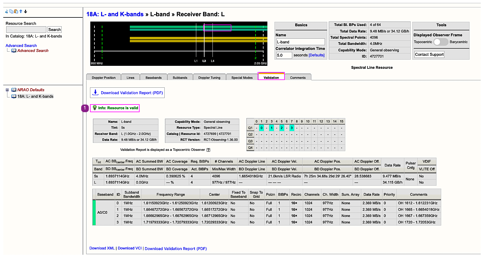
Go to the Validation tab.

Figure 27: Validation Tab: Check to see if resource is valid or not. (Click to enlarge)

The Validation tab summarizes the resource. When done, return to the catalog by clicking its name or by selecting "<catalog name>" in blue font above the resource and repeat these steps for other spectral line resources, such as the K-band resource explained in the next section.

K-band with Lines and Continuum

You will be repeating most of the steps from creating the L-band resource for the K-band resource. Following the L-band example:

Using the same resource catalog, create your resource via the menu: File → Create New → Instrument Configuration
The Resource Wizard will appear. Check the following settings:
1. Spectral Line
2. D configuration
3. Unique name for resource; here "K H20/NH3 Lines" is used
4. Leave the band set for K-band
5. Click Generate button
The Doppler Position tab will appear, fill in the RA and Dec of the science target
Click on the Lines tab, create your spectral line information fields (see Figure 28)
Click on the Baseband tab, click on Automated Setup
The resource will be generated in 8-bit (see Figure 29) and we want a 3-bit resource; there are three ways to change the resource from 8-bit to 3-bit:
1. In Baseband Options select 3-bit (see Figure 30);
2. From the drop down menu select the 3-bit resource (see Figure 31)
3. Manually set up the resource
There will be a warning window appear when you change the resource, go ahead and click OK.
Notice that the baseband distribution is different between clicking the button (Figure 30) and the dropdown menu (Figure 31); with the drop down menu option you will likely need to adjust the center frequency for two basebands A2/C2 and B1/D1 to optimize the spectral line positioning, or you can go with the setup as created when clicking the 3-bit option, which this tutorial will use.
With the 3-bit option setup, the lines are placed in A1/C1, and the basebands B1/D1 and B2/D2 overlap in center frequency; you could change the center frequency of B1/D1 and/or B2/D2 if desired, but it is OK to leave these two basebands alone.
If you attempt to fill baseband A1/C1 with continuum, you will notice that not all of the subbands are filled; you can shift the continuum subbands in the table below the graphical display of the baseband, or you can add subbands and shift their positions as needed, which was done in Figure 32 to bracket the spectral line subbands with continuum on either side as well as the subband with the lines.
Click on the Doppler Tuning tab to set the Doppler position. The lines are in A1/C1, so check that box and select either of the HN3 lines (see Figure 33).
Click on the Validation tab to ensure that the resource is set up correctly and is valid (see Figure 34).


Figure 28: Spectral Line information fields (Click to enlarge)


Figure 29: Default 8-bit setup created by automated setup (Click to enlarge)


Figure 30: Baseband configuration using the 3-bit selection option


Figure 31: Baseband configuration using the drop down menu option (Click to enlarge)


Figure 32: K-band A1/C1 resource with continuum subbands (Click to enlarge)

When you add a subband to the resource, the subband fills in from the right side and not the left; this is due to how the K-band 3-bit sampler works. Once you've generated the subband, you will have to move it by adjusting the subband center frequency.


Figure 33: Setting the Doppler position (Click to enlarge)


Figure 34: Validating the resource (Click to enlarge)

We have created the required resources for the observation and are now ready to make a Scheduling Block (SB) in the OPT using the information we have entered in the SCT and the RCT. Click on the Observation Preparation link at the top to access the OPT.

Create a Scheduling Block in the OPT

About a month before the array configuration begins, proposers will receive an email that their project(s) have been made available in the OPT and are now ready for Scheduling Block (SB) creation. The Program Block (PB) will contain the allocated time for a particular configuration and scheduling priority. This tutorial example was allocated 2.5 hours. For learning purposes, it may be that you need to create your own Test Project within the OPT. You may do so by selecting from the menu File → Create New → Test Project and give the Test Project any name descriptive to you.

The PB should contain an empty SB in which the observer can create the observing scans (see Figure 38). You can rename the SB by selecting it and entering a descriptive name such as "NGC2371 OH H2O NH3". Note that some characters are not allowed in the naming, such as a comma or colon. The PB can also be renamed.


Figure 38: The Project (P, orange) tree in the OPT, with a Program Block (PB, blue) and a Scheduling Block (SB, green).

The SB contains science scans, particularly loops (fast switching between the complex gain calibrator and science target source(s)) and other calibration (flux density, reference pointing, polarization, etc.) scans. The order in which they are created is not too important as long as they adhere to the requirements for observing. This example starts with the science scans before the overhead of the setup scans for the resource(s).

With the version upgrade to 1.28 for the OPT suite of tools, there are new icons in the tree structure that you may see while creating the SB, specifically icons with an exclimation point (!) or a question mark (?). Please see the OPT Manual section on SB Validation Icons for further details and the meaning of these new icons.

Things to Consider:

When observing multiple frequencies, start with high frequency resource(s), in case weather and/or atmospheric phase conditions deteriorate during the observation;
High frequency observing requires reference pointing scans;
Perform flux density and bandpass calibration (polarization is not in this tutorial example);
Complex gain calibrator and science target cycle time (fast switching) loops — 20 minutes for L-band and 7 minutes for K-band for D-configuration;
Anticipated L-band on-source time is 15 minutes (1 loop), K-band 1 hour 45 minutes (15 loops) for this project observation;
Switching between 8-bit and 3-bit requires 30 second requantizer gain setup scans;
Begin with the flux density calibrator (3C48 for this observation) at the start of the SB.

Note that there are different ways to create the SB. All SBs (must) include a start-up phase, a basic science observing component and other required overhead. It is a matter of preference how to get started; different guides may give different suggestions, i.e., building from the beginning of the observations with the initial overhead sequence or start setting up the target-calibration loops with the science in mind. Here the latter is chosen: to start with the science-focused scans and add/insert the overhead later on before the final fine-tuning (which always comes last).

Basic SB Outline

To create our science scans, we start with the simpler L-band observations. We want 15 minutes on source and can use a much longer cycle/loop time between the calibrator scans. However, we should also make sure the individual scans do not get too long (less than or equal to 15 minutes in total duration). We will set up one basic L-band loop: calibrator scan - target scans (two 7.5 minute scans totaling 15 minutes) - calibrator scan. Note that these can also be done without a loop. However, by placing them in a loop it is easier to copy/paste the combination of scans as a whole instead of moving each scan around separately later in the process.

Creating looped scans is done by selecting the SB and then selecting from the menu File → Create New → Scan Loop → In, followed by selecting from the menu File → Create New → Scan → In, to create the first scan within the loop (see Figures 39 and 40). This last step may also be done by clicking on the Page icon (second icon at the top of the left-hand column).


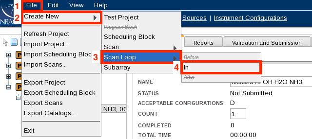Figure 39: Creating a loop.


Figure 40: Creating a scan within the loop.

Within the [New Scan] entry fields, click the Import button in the Target Source field; this will bring up the VLA catalog by default. Select the calibrator you want to use for this tutorial, J0741+331. Rather than scrolling through the entire list of calibrators, you may select the RA position to narrow the search (in this case RA 07, see Figure 41A).


Figure 41A: Importing a calibrator source.

With the OPT 1.31 release there is the ability within the scan to be able to filter the results. As seen in Figure 41A, you have to scroll a fair distance within the RA 07 sources to find J0741+3112. However, if you click on the option to Filter Sources, you are presented with the display as seen in Figure 41B. You click on import (1) as above, then click on Filter Sources. A new window appears that allows you to refine your search. You still need to enter a Source Catalog (2) and a Source Group (3 - if there is one). You can then enter a name of a source (4), or the RA and Dec of a known source, or do a radius search of n degrees based upon the RA and Dec positions. The filtered results are then displayed and you can select the source you want (5). Finally, click on Change (6) to import the selected source.

Figure 41B: Using the filter to import a calibrator source.

To import the resource, click the Import button in the Hardware Setup field, select the project's resource catalog, and there you will see the L-band spectral setup you created (see Figure 42). Note that with the 1.31 release you have the option to also filter the Resources by observing band and/or sampler setup. This is useful if you have a large resource catalog to work through. For this example we only have two sources to choose from, so filtering the resource list makes no sense.


Figure 42: Importing a resource from project catalog.

To finalize this calibration loop scan, select the "Calibrate Complex Gain (A and P)" intent, and uncheck the "Observe target" since this is a calibrator, and set the scan length to a reasonable LST duration (e.g., 1 minute).

The next scan, for the science target, can be created by clicking the Page-+ icon (the third icon at the top), which copies the scan into a new scan with the hardware setup and source from the previous scan. Change the source to the science target by selecting your source catalog in the dialog box and adjust the Scan Timing to 00:07:30 Duration (LST) (see Figure 43). Note the Observe Target intent is the default scan intent. If you make a mistake, a scan or an entire SB can be deleted or cut by selecting it and clicking on the Scissors icon (the fourth icon at the top).


Figure 43: A science target scan.

To duplicate the science target scan, click on the Copy icon (the fifth icon at the top), and paste it with the Paste icon (sixth item at the top) to increase the duration of the science target to twice 7.5 minutes. Finally, select the calibrator scan and copy/paste it to the last scan in the loop, this time by selecting from the menu Edit → Copy STD: J0741+3312, then click the last scan and select from the menu Edit → Paste After STD: NGC2371 (see Figures 44 and 45).


Figure 44: Copy scan STD: J0741+3312.


Figure 45: Paste After scan STD: NGC2371.

Now we will create a similar loop in K-band, and place it so it is observed before the L-band scans.

Select the L-band loop (rename it to "L-band loop" or something descriptive) and select from the menu File → Create New → Scan Loop → Before, and give the new loop a name, e.g., K-band loop. Since we want the K-band loop to run 15 times, set the Loop Iterations to 15 (see Figure 46).


Figure 46: The K-band loop settings.

In the K-band loop we want to create a science target scan of 7 minutes and a complex gain calibration scan of 1 minute, similar to the steps for the L-band loop, except using the K-band resource that was created for the Hardware Setup.

Since K-band observations require reference pointing calibrations, place another complex gain calibrator scan before the K-band loop (see Figure 47). Be sure to import the K-band setup for the Hardware Setup and use the "Calibrate Complex Gain (A and P)" scan intent for the complex gain calibrator scans.


Figure 47: Filling the K-band loop.

Because K-band is high frequency, we will be adding reference pointing scans (see below). We will select the Apply Last Reference Pointing setting for all K-band scans, except for the pointing scan itself. Note we can extend the complex gain calibrator scan before the loop and use it as a bandpass calibrator if we decide to do so. However, 3C48 is bright enough and does not differ much in flux density with this source in K-band, so we will use 3C48 for bandpass calibration and benefit from the known spectral slope of this standard flux calibrator in determining the bandpass.

Before the first calibrator outside the loop, we need to add a pointing scan (see Figure 48). And because we are switching from 8-bit to 3-bit after the pointing, another setup scan is required. We add two scans of the calibrator: the first scan should be a pointing scan with scan mode selected to be Interferometric Pointing and an initial duration of 3 minutes (may need to be increased later) using the X-band pointing resource from the NRAO defaults catalog and the pointing target (which fortunately again is J0741+3112). Furthermore, make sure there is no "Apply Last" selected in the reference pointing column.


Figure 48: The Reference pointing scan using the complex gain calibrator source with the adjusted time on source of 7 minutes.

The second scan, which is another setup scan after the 8-bit resource pointing scan but before the 3-bit K-band gain calibration scan, should apply pointing and use the K-band resource with a setup intent for a duration of 30 seconds (see Figure 49).


Figure 49: The basic science scan sequence starting with the pointing scan and the requantizer setup scan before the gain calibration scan.

Start-up Overhead

Figure 49 shows the science part of the observation. Now we should allow for the start-up overhead, flux density, and bandpass calibration. The flux/bandpass calibration is best placed at the start or at the end of the observation as it typically requires long slews away from the region of interest. Here we chose to do flux density calibration at the start of the observation using 3C48. Other examples are given in the extensive documentation throughout the OPT manual and the Guide to Observing with the VLA. The sequence to follow from the start of the observation to the first science scans is as follows:

Default Resource Setup at the Start	Scan Time	Intents and Notes
L-band setup on first source (3C48)	3 minutes	setup scan (set 8-bit attenuator levels)
K-band setup on first source (3C48)	1 minute	setup scan (set 3-bit attenuator levels)
X-band pointing setup on first source (3C48)	1 minute	setup scan (set 8-bit attenuator levels)

Flux and Bandpass Calibrator Scans	Scan Time	Intents and Notes
X-band reference pointing on 3C48	7 minutes	Interferometric Pointing scan mode; Start-up includes initial setup scans plus the first calibrator or reference pointing scan to allow 10-12 minutes in total duration. When starting with reference pointing, a 12 minute (minimum) start-up is the best approach.
K-band 3-bit setup on 3C48	30 seconds	setup scan (setting requantizer levels) when switching from 8-bit (X point) to 3-bit (K), apply last (reference pointing)
K-band bandpass and flux on 3C48	a few (3) minutes	flux density scale, bandpass, complex gain, apply last (reference pointing)
L-band bandpass and flux on 3C48	a few (3) minutes	flux density scale, bandpass, complex gain, apply last (reference pointing)
Science scans to follow		science target bracketed by the complex gain calibrator

If the four flux density and bandpass scans are moved to the end of the observation, the resource setup at the start would be using the pointing source and an additional pointing scan on that source for 7 minutes. Examples can be found in the OPT Manual and the Guide to Observing with the VLA. The sequence in the table above is shown in Figure 50.


Figure 50: The resource setup and flux and bandpass scan overhead at the start of the observation, before the basic science scans.

Now that the observing structure is in place, click on the SB name to enter the scheduling parameter within the Information tab. In the hypothetical proposal for this project, the LST range for this source to be above 25 degrees elevation was calculated to be between 02h16m and 18h51m. The earliest LST start time for this observation is 02h16m, but as this block is 2.5 hours long, the latest LST start time is 16h31m (which follows from the latest LST allowed, 18h51m, minus 2h30m for the length of the block). Enter this in the Information tab for the LST start range (02:15 and 16:30). Finally, select the weather conditions for the highest frequency band used in the SB (K-band), i.e., 7 m/s for wind and 10.0 degrees for the API upper limits to start this SB (see Figure 51).


Figure 51: The dynamic scheduling starting conditions for this SB for LST start range and weather for the highest frequency band in the SB. The set up scans for slew to area of sky and attenuation set up are the scans in the red block; reference pointing scans and flux density / bandpass calibration scans are in the blue block; complex gain calibration and science target scans are in the green block. (Click to enlarge)

Fine Tuning

Click on the Reports tab to see how this SB would perform for the average start time (12:52:30, or any other time selected within the assumed LST start range on the Reports tab). The window at the bottom will show an error and the scan listing (third table down the main window) will show many red rows (see Figure 52).


Figure 52: The scan rows in red indicates an error condition with the scan (source elevation below the horizon).

For the first scan, and the setup scans to follow, this is normal and nothing to worry about; but it should be clear that for the assumed starting time of 12:52 LST that 3C48 has already set below the horizon. The Guide to Observing with the VLA shows that 3C48 is only up until about 08:33 LST for the minimum elevation limit (10 degrees), and will be below the anticipated 25 degrees elevation limit after about 07h LST. Return to the Information tab and use 06:40 as the latest LST start (to account for the first 20 minutes of time spent on 3C48), and go back to the Reports tab. Another error appears, this time on the pointing scan which requires 2:30 minutes on source after any necessary slewing. We allocated a duration of 3 minutes, but more than 30 seconds is spent on slewing from 3C48 to the first source (see the red scan row in Figure 53).


Figure 53: The reference pointing scan on J0741+3312 is too short to perform the antenna pointing.

In this particular case the software chooses the shortest way, clockwise (CW), to go from Az 280° (where 3C48 is at the LST start time) to the rising gain calibrator at Az 440°. The antenna array should be directed counter-clockwise (CCW) to make this slew happen from Az 280° CCW to Az 80°(=440°). To achieve this, select CCW wrap for the relevant (8th) scan (see Figure 54) on the gain calibrator and add about 5 minutes to the total time to allow for a 200° slew at 40° a minute (the Azimuth slew rate of the telescopes). These errors are now gone in the Reports tab, and ample time is left for the pointing scan.


Figure 54: Selecting the wrap for a scan.

Try other LST start times in the start range, watch for errors on particular scans, and fix them if they appear. Make sure to stay within the allocated time (2h30m) and modify the schedule, if necessary, to achieve this criteria. In this case the total time is 2:45 so 15 minutes must be cut, for example, by taking 40 seconds off the K-band target scan and 20 seconds off the K-band calibration scan (one minute per loop, 15 loops). Other choices are also possible as long as you can still detect your calibrator and perform other calibration scans. Go back to the Reports tab and play around with LST start times and look for errors, e.g., short on source times (less than 20 to 40 seconds). Finally, go to the Validation tab, validate and submit (Figure 55).

Note that with the release 1.31 there is an option for you to opt out of COSMIC-SETI (information on COSMIC-SETI). By default this box is always checked, meaning that COSMIC-SETI will get the raw data plus the metadata (source name, position, observing frequency, etc.) from your observing. Opting out means that while COSMIC-SETI will still get the raw data, none of the metadata are provided, which renders the raw data useless.


Figure 55: The Validation tab. (Click to enlarge.)

If you have problems that you cannot fix yourself or with help of a colleague, please feel free to ask the NRAO Hepdesk.