How to Propose

Observing time on the VLA is available to all researchers, regardless of nationality or location of institution. There are no quotas or reserved blocks of time. The allocation of observing time on the VLA is based upon the submission of a VLA Observing Proposal using the online Proposal Submission Tool (PST) available via the NRAO Interactive Service web page, at https://my.nrao.edu/. The online tool permits the detailed construction of a cover sheet specifying the requested observations, using a set of online forms, and uploading of a PDF format scientific justification to accompany the cover information. More specific info on using the online tool, and policies related to proposal types, scientific justification page limits, etc..., can be found in the NRAO User Portal and Proposal Submission Guide. VLA-specific details, including capabilities offered for the next proposal deadline, can be found in the Offered VLA Capabilities chapter of the current VLA Observational Status Summary (OSS) document. For further information on observing at the VLA, including information on radio frequency interference (RFI), 8/3 bit Attenuation and Setups, and pre-submission checklists for Scheduling Blocks and instrument configurations, please see the Guide to Observing with the VLA.

It is also possible to obtain VLA observing time by proposing to NASA missions, under cooperation agreements established between NRAO and those missions. Such programs exist for the Chandra, Fermi, Swift and HST missions. Astronomers interested in those joint programs should consult the relevant mission proposal calls for more information.

Note that it is possible to search cover sheets of proposals previously approved for time using the Proposal Finder Tool (PFT).

Students

Students planning to use the VLA for their Ph.D. dissertation must submit a Plan of Dissertation Research of no more than 1000 words with their first proposal. This plan can be referred to in later proposals. At a minimum, the plan should contain a thesis time line and an estimate of the level of VLA resources needed. The plan provides some assurance against a dissertation being impaired by an adverse review of a proposal when the full scope of the thesis is not seen. The plan can be submitted via NRAO Interactive Services. Also see the Plan of Dissertation Research subsection of the NRAO User Portal and Proposal Submission Guide for more details. Students are reminded to submit their plan comfortably in advance of the proposal deadline. New thesis plans must be in PDF format to enable science reviewers to easily access the plans. Students who have not yet graduated, but have active plans on file, should consider updating those plans to a PDF format if they are not already in that form.

Timeline

Time on the VLA is scheduled on a 6-month semester basis. Semester A observations typically take place February through July and have an August 1 proposal deadline in the previous year; Semester B observations, with deadline February 1, take place from August through January. If the deadline falls on a weekend it is extended to the next working day. The call for proposals, which typically goes out 3–4 weeks prior to the deadline, includes an overview of upcoming deadlines and VLA configurations.

For details on the evaluation of submitted proposals we refer to the NRAO Proposal Evaluation/Time Allocation page. Because of competition, even highly ranked proposals are not guaranteed to receive observing time. This is particularly true for proposals that concentrate on objects in the LST ranges occupied by popular targets such as the Galactic Center or Virgo. Daytime VLA observing will also continue to be limited by ongoing testing and maintenance activities; for more information, see the section on Scheduling Considerations in this document.

Director's Discretionary Time

It is also possible to propose for Director's Discretionary Time (DDT). DDT is reserved for Targets of Opportunity and for Exploratory Time. DDT proposals may be submitted at any time with the understanding that they should only request for the current and, maybe, the next upcoming array configuration. The DDT proposals must be submitted through the PST. DDT proposals are reviewed by Observatory scientific staff on the basis of the proposals' scientific merit, conflict status, LST pressure, and technical feasibility.

Introduction

The VLA is reconfigurable and uses all antennas in a single array in four principal array configurations, A through D; the antennas can also observe in multiple sub-arrays as discussed below. The A-configuration provides the longest baselines and thus the highest angular resolution for a given frequency, but yields very limited sensitivity to surface brightness. The D-configuration provides the shortest baselines, translating to a high surface brightness sensitivity at the cost of angular resolution. See the configuration schedule for details for each call for proposals and the highest angular resolution as function of frequency in the OSS. In general, as the baseline length expressed in wavelengths gets longer, the phase stability gets worse which impacts the observing strategy and observing overhead.

It is generally important to consider the following:

• What angular resolution is required for the proposed science at the desired observing frequency?
• For resolved sources, how does the desired angular resolution compare to the required surface brightness sensitivity?
• For the array configuration that gives the desired angular resolution, how much of the flux density is actually in compact components, and will not be resolved out?

The Observational Status Summary section on Resolution, in conjunction with the Exposure Calculator, can help answer these questions.

Please note that low declination sources risk being subject to antenna shadowing at certain azimuths for the C and D configurations. These targets can still be observed. Observing at low declination implies, however, smaller windows of no-shadowing (one on either side of the north-south arm), which effectively makes the setup of the scheduling blocks harder or the observation less sensitive than expected.

Note on hybrid configurations: For very southern (and very northern) declinations, the VLA used to offer hybrid array configurations where the north arm was extended compared to the east and west arms. This provided a more circular synthesized beam at declinations south of −15 deg and north of 75 deg, at the cost of limited scheduling opportunities due to the short duration of the hybrids. Semester 2016A was the last semester to offer the hybrid configurations. See the following section for alternatives to the hybrids.

Alternatives to Hybrid Configurations

The approach required to substitute for the lack of hybrid VLA configurations depends on the science goal and observing mode of a proposal as described below. We assume projects that would have proposed to use the hybrid configurations are requesting them because they wish to observe sources at southern (<−15 deg) or northern (>75 deg) declinations.

Point Sources

Proposers should request the next largest principal configuration and ask for the same amount of observing time that would have been requested in a hybrid.

Extended Structure

Good surface brightness sensitivity is needed for projects aiming to image an extended structure. The surface brightness sensitivity of a hybrid configuration can be reproduced by:

- either doubling the on-source integration time of the next largest principal configuration, or;
- combining 1.0 × (larger configuration) + 0.4 × (smaller configuration).

The choice of which to use depends on the science goal, declination, and observing mode, as described below. An exception is the DnC hybrid, for which shadowing at very low declinations makes the use of the D configuration very inefficient. To substitute for the DnC hybrid, proposers with targets at δ<-25 deg should always request double the amount of DnC observing time in C configuration.

• Imaging extended structure with on-source integration times of around a minute or more:

1. CnB/BnA substitute: proposers should combine 1.0 × (larger configuration) + 0.4 × (smaller configuration).

• Note: if the field contains variable sources, but the science goal is imaging of extended structure, proposers should either request double the time in the next largest principal configuration (if this can be accommodated in a single scheduling block), or be prepared to model and subtract variable sources from individual datasets prior to combining, as needed.

• Imaging extended structure with very short on source integration times (e.g., large mosaics): very short scans can result in large slewing overheads, so to optimize observing efficiency proposers should request double the on-source time that would have been requested in the associated hybrid, for the next largest principal configuration.

For more details on how to optimize the science on the VLA without the hybrid configurations, as well as technical details regarding the above noted recommendations, we refer to the EVLA memo 193. Also, proposers should direct any questions about which configuration they should use to the NRAO Helpdesk. For an example on how to combine data from several array configuration, we refer to the VLA data combination guide.

Solar Observations

The Sun is a very extended source and has a complex brightness distribution that varies in time due to solar rotation and intrinsic source variation. For this reason, only a single configuration should be used to observe the Sun rather than combining different configurations. Furthermore, time variable phenomena such as flares require the use of the instantaneous, or snapshot, uv coverage provided by a configuration. The most useful configurations for observations of the Sun at frequencies above 1 GHz are the C and the D configurations. The A and the B configurations provide coverage that is too dilute and that over-resolves the Sun.

Subarray Observations

Instead of using all (27) antennas to observe one source using one resource at a time, the VLA can also be split in groups of antennas observing different sources or with different resources simultaneously. The drawback is of course that the fewer antennas in a subarray are less sensitive per unit time, and provide fewer baselines, fewer u,v data points, and thus a sparser sampling of spatial frequencies for image reconstruction. However, many science programs are quite suitable for using sub-arrays, for example bright point sources for which one desires exactly simultaneous observations at different frequency bands, possibly with similar angular resolution, or when surveying a large sample of sources using only half or one third of the observing time.

There are some restrictions in how to set up the correlator or divide the antennas over the sub-arrays as explained in the Observational Status Summary and requesting sub-arrays in the Proposal Submission Tool (PST) is not exactly straightforward. For the latter we provide some guidelines here:

In the PST, there are five items to pay attention to: a check-box on the cover sheet, the list of sources, the resources, the sessions and the fill-out box in the technical justification.

• Cover sheet: under the "General" item in the proposal there is a subsection for "Observing Type(s)". Tick the relevant items, including the check-box in front of "VLA Subarrays"
• Sources: for each of the sub-arrays you would want to define a separate source group, unless you observe exactly the same sources in each sub-array.
• Resources: for each of the sub-arrays you would want to define or select (from the defaults) a separate resource, unless you want to use exactly the same resource in each sub-array. Note that if you use the same sources you typically want a different resource per sub-array and vice-versa.
• Sessions: this may get a bit tricky as it is impossible to get the total time right with your intended use of sub-arrays. Currently the PST simply sums up the times requested per sub-array, which means it over-estimates the requested total time in the proposal by a factor of N_sub, where N_sub is the number of sub-arrays. For General Observing, N_sub can be up to 3. The easiest way to overcome this limitation in the PST is to divide your total requested time (T_tot) by the number of sub-arrays (N_sub) and use that number as follows: 
  
  1. Make a session with a source group and a resource,
  2. Fill in the time per session as T_tot/N_sub, 
  3. Save the session,
  4. Click "Add" to the right of  "Time/Session (hrs)" - you do not click on "New Session" at the top right,
  5. Define a new component to that session with a source and resource, and again a session time of T_tot/N_sub, save, click "Add", until you have defined N_sub components in that session, which now should add to the total requested time T_tot on the cover sheet. 
  Claiming 1/N_sub for the session time per sub-array is in effect equivalent to asking for the total time T_tot per sub-array but only for 1/N_sub part of the full array. It is because the latter is not implemented in the PST, the steps listed above are the work around. If, however, these steps are not followed and for each sub-array T_tot time is requested, then the total time request on the cover sheet will be reflected as T_tot*N_sub. This will be wrong, and will in turn raise questions/concerns during the review process.

• Technical Justification: in the dedicated text box for sub-arrays, you will need to explain the use of sub-arrays and what has been done to the sessions to get to the total requested time. Also, add any other relevant technical details as needed.

Sessions

Scheduling priorities for the VLA are based on the use of sessions in the PST, which are the units of observing time considered by the Time Allocation Committee. Since the observing priority assigned to a session can strongly depend on how the proposer structures these sessions, we provide a set of guidelines to help you in defining your sessions.

High Frequency

High frequency observations are susceptible to atmospheric effects, such as air turbulence and water vapor. During the summer months, and especially during daytime, conditions appropriate for high frequency observing are limited. Other limitations may include needing night-time observing or observing during dry seasons for increased phase stability. With the stricter weather constraints on high frequency (> 15 GHz) observations, programs are in competition for less available time. Figure 3.1 illustrates a sample plot showing the fraction of available days, as a function of LST, for observing at various bands in April 2011.

Figure 3.1: The fraction of days where conditions are suitable for various frequency bands as a function of LST derived from actual data in April 2011. Note the smaller fractions of time available for the higher frequency bands at certain times. Projects requiring LSTs during which this fraction is small for a given band are less likely to be observed. In this particular example, high frequency projects are less likely to be successful in the LST range 0–8h. Note that the available time is further decreased by daytime maintenance activities. We provide summary plots for other months at Monthly Conditions at the VLA.

For more information on high frequency observations, please see the High Frequency Strategy section of the Guide to Observing with the VLA.

Low Frequency

Observations using the lower frequency bands of the VLA may be adversely affected by Radio Frequency Interference (RFI). There is extensive documentation on RFI at the VLA. Please see the Radio Frequency Interference section in the Guide to Observing with the VLA. Furthermore, such observations may be impacted by solar activities that can cause disturbing ionospheric effects. For more details, see the Low Frequency Strategy and the Very Low Frequency Strategy sections of the Guide to Observing with the VLA.

LST Range

For a number of reasons, the observer might prefer night-time observing over daytime observing:

• During the night, phase stability tends to be better, which is important for high-frequency observing, and there is no solar interference which could affect low-frequency observing.
• There is less time available for observing during the day because of scheduled maintenance and testing on most weekdays, and a session with sources visible only during the day may end up with lower observing priority than when its sources are up during the night.

Figure 3.2 shows the daytime LST range as a function of the day of the year, which can assist you in planning your observations. We note that for moving sources, such as planets, the situation becomes more complex as their LST range suitable for observing tends to vary during the course of the year.

Other considerations to account for are the elevations of the sources within the following limits: Minimum elevation of 8 degrees (hard limit); Minimum elevation of 10 degrees for low frequency, 20 degrees for high frequency and S-band; Maximum elevation of 80 degrees for high frequency, 85 degrees for low frequency. And for programs that require a considerable amount of observing time at a specific LST, how much time is actually available and does the program request more than a few percent of that? More information on times of high and low observing pressure by LST can be reviewed in the Call for Proposals.

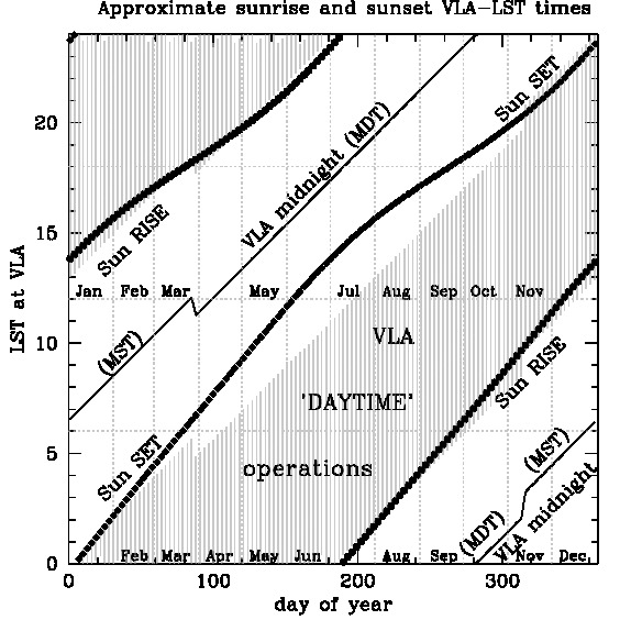Figure 3.2: The location of sunrise, sunset, and (shaded) potential test/maintenance time as a function of time of the year and LST.

Moving Objects

The VLA is able to observe moving objects (solar system bodies) in standard continuum modes as part of general observing. It is not currently possible to observe spectral lines in planets or comets, except in unusual circumstances (background source occultations, for instance), or as part of the Resident Shared Risk Observing (RSRO) program.

Also be aware that during the configuration, moving objects may be observed at LST ranges that are considerably different between the beginning and ending date. Please indicate in the proposal when the optimum date ranges are, and what LST ranges they correspond to. It is beneficial to avoid the high-pressure LST ranges if the object can be observed at other times. For extended objects, also comment on the largest angular scales necessary in the imaging and what date ranges need to be avoided as the object would be too close/large.

For more information on observing moving objects with the VLA, please see the Moving Objects section of the Guide to Observing with the VLA.

Solar Observations

Solar observations typically request that specific types of solar phenomena or activity are present on the solar disk at the time of observations. Assuming that the project has sufficiently high scheduling priority, solar observers must therefore communicate closely with the VLA scheduler to ensure that they are aware when promising targets are available. Solar observations can usually be scheduled 2-3 days in advance.

Sun Avoidance

Throughout the course of the year, the Sun moves across the sky with respect to background objects. Due to the NRAO's use of dynamic scheduling, a scheduling block may end up being observed when the Sun is close enough to have an adverse effect on the data with phase fluctuations and elevated system temperatures.

Please see the section on Avoiding the Sun in the Guide to Observing with the VLA. There is an online tool available to check and see how close your sources are to the Sun and Moon; here is the link to the VLA Sun & Moon Distance Check Tool.

Frequency Bands

All VLA antennas are outfitted with eight cryogenically cooled receivers providing continuous frequency coverage from 1 to 50 GHz. These receivers cover the frequency ranges of 1–2 GHz (L-band), 2–4 GHz (S-band), 4–8 GHz (C-band), 8–12 GHz (X-band), 12–18 GHz (Ku-band), 18–26.5 GHz (K-band), 26.5–40 GHz (Ka-band), and 40–50 GHz (Q-band). Additionally, all antennas of the VLA have receivers for lower frequencies, enabling observations at both P-band (200–500 MHz) and 4-band (54–86 MHz).

For more information on frequency bands and tuning, please see the VLA Frequency Bands and Tunability section in the VLA Observational Status Summary.

Samplers

The VLA is equipped with two different types of samplers: 8-bit with 1GHz bandwidth each and 3-bit with 2GHz bandwidth each.

The 8-bit set consists of four 8-bit samplers arranged in two pairs, each pair providing 1024 MHz bandwidth in both polarizations. The two pairs are denoted A0/C0 and B0/D0. Taken together, the four samplers offer a maximum of 2048 MHz coverage with full polarization. The frequency spans sampled by the two pairs need not be adjacent. Some restrictions apply, depending on band (e.g., the Ka-band), as described in the section on Frequency Bands and Tunability.

The 3-bit set consists of eight 3-bit samplers arranged as four pairs, each pair providing 2048 MHz bandwidth in both polarizations. Two of these pairs, denoted A1/C1 and A2/C2, cannot span more than 5000 MHz (lower edge of one to the higher edge of the other). The same limitation applies to the second pair, denoted B1/D1 and B2/D2. The tuning restrictions are described in the section on Frequency Bands and Tunability. Taken together, the eight 3-bit samplers offer a maximum of 8192 MHz coverage with full polarization.

For more information on samplers and which set to use, please see the VLA Samplers section in the VLA Observational Status Summary.

The correlator configuration depends entirely on the science goal. For continuum science, choose the widest bandwidth per subband with coarse spectral resolution; typically the NRAO default settings (possibly retuned to alternative center frequencies) are sufficient. For spectral line, choose the subband bandwidth and the spectral resolution that best fit the scientific objectives of your project. For pulsar observations, spectral resolution and pulse phase (bin) resolution should generally be chosen to maximize bandwidth while still resolving the pulse; your project may have other specific requirements depending on the goals.  Detailed information on the correlator is available in the WIDAR section of the VLA OSS.

Issues that should be kept in mind are:

General and Spectral Line Considerations:

• The widest (128 MHz) subbands in a baseband do not overlap. Additionally, a few channels may need to be flagged at either subband edge because of the higher noise due to filter roll-off. If the science goal requires a homogeneous sensitivity sampling over multiple 128 MHz subbands, we recommend tuning the second baseband at a frequency that is offset by a fraction of a subband width with respect to the first baseband. This, however, removes the possibility to place the second baseband freely in the receiver band to do other science. Also, anywhere from 8 MHz to up to 30 MHz at the edges of the basebands may be noisier, so you should not rely on a spectral line that would be close to a baseband edge. For more details, see the Subband 0 subsection of the Spectral Line section in the Guide to Observing with the VLA. 

• As described below, each subband must be calibrated independently. Therefore, in the case of a narrow subband bandwidth, choose flux density and complex gain calibrators that are strong enough for adequate S/N at this subband bandwidth. For more information about successful calibration, see the Exposure and Overhead in this guide, and the Calibration section in the Guide to Observing with the VLA.

• It may be necessary to Hanning smooth your data in order to get rid of Gibbs ringing (for the theory behind this phenomenon see Gibbs phenomenon). Lower frequency bands (X and below) are prone to strong Radio Frequency Interference (RFI); flagging the RFI could be close to impossible unless you first Hanning smooth your data. This necessity should be taken into account when choosing the spectral resolution of your proposed observations, since the effective resolution will be lower than the original (pre-Hanning smoothed), even though the number of channels will stay the same. Note that the frequency resolution (FWHM) of un-tapered spectra is 1.2×Δν (where Δν is the channel spacing) and the resolution of Hanning-tapered spectra is 2.0×Δν .

• For spectral line observations, given an expected line width, it is a good idea to select a spectral resolution that will allow for at least 4–5 channels across your line, or twice that many when Hanning smoothing. There are a number of tools available online to identify molecular line rest frequencies such as the Lovas Catalog and Splatalogue. The frequency range covered by ~10 to 50 GHz (X to Q-band) contains a large number of diagnostically interesting atomic and molecular transitions. For continuum data only, it is wise to check whether the chosen frequency range contains potentially strong spectral lines.
• Any correlator configuration should stay within the allowed data rate limits for GO and SRO observing. This might become an issue with complex correlator setups using recirculation and/or short integration times. GOST will report the data rate for a specific correlator setup.
• Spectral line correlator configurations are typically set up with GOST (see next section) in the proposal stage (PST) and with the Resource Catalog Tool (RCT) in the OPT for the actual observations. GOST however may not handle all configurations correctly, in particular the case of using 32 subbands in a baseband and for P-band spectroscopy. In such cases, the PST will accept screen shots of the configuration as shown in the RCT. See at the end: "If GOST Fails".

Pulsar Observations:

• There are two different pulsar observing modes available at the VLA:  phased-array (also called "YUPPI" mode) and phase-binned imaging mode. 
• In the phased-array mode, the individual antenna data streams are summed coherently in real-time to produce high time resolution data on a single sky pixel.  Coherent de-dispersion can optionally be applied, and the data can be written out either as high-time-resolution spectra, or folded modulo a known pulsar timing ephemeris.  See the Pulsar Observing section of the OSS for more details.
• In phase-binned imaging, the antenna cross-correlations (visibilities) are averaged into different pulse phase ranges using a known pulsar timing ephemeris.  This gives data for the entire field of view, but generally with much worse time resolution than is available in phased-array mode.
• For phase-binned pulsar observations, there are constraints and trade-offs between the total number of subbands and the bin width.  There is also an output data rate limit that will affect the maximum number of bins allowed for a given dump time and number of channels.  These issues are described in more detail in the Pulsar Observing section of the OSS, under the "Gated or binned visibilities" heading.  The Resource section of the PST will prompt for the relevant information and compute the data rate for pulsar binning modes.
• In general for pulsar binning observations, the bin width (via number of bins) should be chosen to be comparable to or smaller than the pulse width.  The spectral resolution (via subband bandwidth) should ideally be chosen so that dispersive smearing within a channel is comparable to or smaller than the bin width.  Dispersive smearing can be computed as Δt_DM = 8.3μs x Δν(MHz) x DM(pc cm^-3) / ν(GHz)³.
• Dump time for pulsar binning should generally follow standard guidelines for interferometric imaging (see for example the Field of View OSS section).  Binning observations require the target source to have a known timing ephemeris, in TEMPO-compatible format.  The ephemeris does not need to include absolute phase information, but it should be accurate enough so that the pulse phase drift (due to any apparent pulse period error) within a dump time is much smaller than the bin width.

The General Observing Setup Tool (GOST)

Introduction

The General Observing Setup Tool (GOST for short) is used at the proposal planning stage to specify the anticipated correlator configuration and resources to be used in conjunction with the proposed Karl G. Jansky Very Large Array (VLA) observations.

GOST is a Java application and is updated for the expected capabilities per VLA observing semester as advertised in the Call for Proposals (CfP, see the current OSS). The use of GOST is required for non-default continuum and spectral line observations in order to ensure that planned correlator setups and data rates comply with the capabilities offered for each VLA observing semester. Proposers who define spectral line correlator configurations must ensure that such configurations are, in fact, allowed and that these configurations are correctly communicated to those reading the proposals. GOST helps determining whether a setup is (in principle) possible and whether it falls under Standard, Shared risk, or Resident shared risk observing.

The tool enforces most of the known hardware limitations, such as on the number of subbands and number of channels, but does not include the detailed frequency setup for all subbands. GOST does not replace the careful validation that, including the detailed frequency configuration setup checking, is done in the Resource Catalog Tool (RCT). Note that if a correlator configuration can be configured in GOST, it does not mean that it is wise, or that considerations and restrictions outside the correlator are not equally or even more important. If in doubt, create the full setup in a test resource and validate it in the RCT and/or consult the NRAO Helpdesk.

Proposers must attach the output of this program as a screen snapshot for each of the possible line setups used in the proposal to communicate their intent to the reviewers and the Time Allocation Committee. Continuum and Resident shared risk (RSRO) configurations do not require GOST. Default Continuum resources are integrated into the Proposal Submission Tool (PST) and therefore can be selected directly. RSRO configurations must be described in detail in the appropriate sections of the proposal's Technical Justification.

In the near future it is anticipated that GOST will be replaced by actual resources as defined in the RCT. The RCT is part of the Observation Preparation Tool (OPT).

The rest of this document describes running GOST. For capabilities, definitions and other proposing and observing related content please see the current VLA Observational Status Summary (OSS), the Guide to Proposing for the VLA, the Guide to Observing with the VLA, the Proposal Submission Tool (PST) manual, and the NRAO and VLA science web pages in general. For missing or confusing documentation, etc., please contact the NRAO Helpdesk with your queries and/or suggestions.

Starting GOST

GOST should only be used to define configurations for Standard and Shared risk observing in non-default continuum and spectral line mode for observations above 1 GHz. Plain Continuum can be selected as a default mode in the PST; Resident shared risk configurations must be described in text in the proposal. A special case is P-band spectroscopy for which we require a screen shot of the validation page of the Resource as defined in the RCT/OPT.

To run GOST, a current version of Java webStart needs to be available on the host computer. The Java issues page has solutions for potential problems. The interactive GOST Java application can be launched (left click, you might need to do a "javaws -clearcache" in a terminal to get the latest version) or, alternatively, downloaded (right click) as a jnlp-file and selecting Save link as... In the latter case, GOST can be run without an Internet connection from the command line with javaws <downloadDirectory>/latestGOST.jnlp; this has the disadvantage that an older version of GOST may run if it has not been replaced by the newer version. Usually this is not a problem if the jnlp-file is downloaded just before running it.

This is the default view of GOST when first launched (click the images to enlarge in a new tab or window).

Figure 6.1: At the top left hand side there is an option menu (Subbands, View and Help) (see figure left), but more importantly there is a configuration designation in colored font in the top center field (see figure above). At the bottom a Save button will save a screen shot to disk which then should be attached to the proposal in the PST (see figure below). Fields shown in blue font are editable and thus under control of the proposer; fonts in black are derived from the selections made.

Configuration Designation

In the center of the menu bar is a box that contains one of four (five) possible designations for the correlator configuration. The designations are:

For designations other than Standard, the labels of the triggered warnings are displayed in colored bold type with a prefix marker (e.g., "[!]", not shown in subband columns). When this is the case, please use the Why? button (which will appear next to the configuration designation) for more information as to why the software has chosen this designation. It is then left to the proposer to either change the parameters in GOST back to Standard capabilities or to accept the newer designation.

Saving Your Work

Clicking the Save button will save a screen shot of the parameters set in GOST to an image file. Please choose a directory location and a unique name for the image file. The system will automatically append a .png suffix. Save one image file for each configuration to be included in the proposal. The PST will accept these images as attachments to the proposal.

On smaller screens (e.g. laptops) pressing Save in GOST will only save the visible part of the window. If the window does not fully fit the screen, one can use the options under the View menu to adjust the size of GOST: F4 to show only A/C, F5 to show only B/D, F6 to show both A/C and B/D (default). If only a few subbands are filled, one can use the Show Unused Subbands (F7 key) to reduce the size of the screen. Note, however, that the PST only takes a single screen shot as input per resource. If two or more screen shots have to be taken to capture all the information for a resource, one needs to combine them in some other program to a single png before uploading (e.g. in xfig).

Note that GOST parameters cannot be saved! Whenever GOST is re-started, all the input parameters are set to their default values. If several closely-related configurations need to be constructed, do so in a single GOST session, saving a snapshot of each configuration when completed. Exiting the tool will require to start over again from scratch.

Special note for users with multiple monitors. Tests in the past have shown problems with the screen capture mechanism for users who have more than one monitor. After saving a GOST screen shot image to a file, please open that file to ensure it took a correct snapshot. If it did not, try moving GOST to another monitor (tests indicate that the first monitor is more likely to give proper results). If the screen capture does not properly work on any monitor, please use a third party tool to take the snapshot and save it in png format only.

Getting Started

GOST help pages with screen shots follow first. Jump directly to GOST usage hints below.

Spectral Line Input Help

GOST allows VLA observers to concentrate correlator capabilities on several narrow regions of frequency space (i.e., in subbands placed in basebands). The VLA offers two different samplers to the community: An 8-bit sampler with 2 basebands of 1 GHz bandwidth each (A0/C0 and B0/D0 for the two polarization pairs), and a 3-bit sampler with 4 basebands of 2 GHz baseband each (A1/C1, A2/C2, B1/D1, B2/D2). While the 3-bit sampler provides more bandwidth, the 8-bit sampler is better suited for high dynamic range experiments. The 8-bit samplers are, per frequency interval (e.g. for spectral line work), also more sensitive than the 3-bit samplers at any frequency.

For a more detailed description of basebands, subbands, baseline board pairs, etc., and their restrictions for use, please consult the WIDAR section in the OSS, the Spectral line section in the Guide to VLA observing, and the RCT section in the OPT manual.

The baseband setup fields of GOST summarizes the receiver to be used and the global setup of each baseband property. In the lower portion, the subbands tables (up to 2 by 2 sub-tables), summarize the setup of the subband properties in each of the active basebands.

Below follows the description and help for the parameter fields of each of these tables.

Baseband Setup Fields

Figure 6.2: Baseband setup fields: plain 3-bit (top) and 8-bit (bottom) views.

Receiver Band

The observing bands labeled with the receiver names are ordered from lowest to highest frequencies. Choose the one to be used for this setup. Note that at this time 4/P-bands are not included in the drop down as only the default continuum P-band setup is offered as non-shared risk mode. For P-band spectroscopy a screenshot of the RCT is required instead. As 4-band is still RSRO, 4/P-band observing setups do not use GOST.

 

A/C and B/D Basebands

The baseband samplers to be used, either 3-bit or 8-bit. Note that mixed settings no longer result in a Shared risk configuration. 8-bit samplers require one baseband center frequency per polarization pair, 3-bit samplers require two (see Baseband Center Freq. next).

Baseband Center Freq (GHz)

Depending on the chosen sampler, these are the one or two input fields for the baseband center frequencies in GHz for AC and BD each. For 3-bit, note that the A1/C1 and A2/C2 baseband centers must be separated by less than 2.5 GHz; the same also holds for the B1/D1 and B2/D2 baseband centers. For restrictions in absolute baseband center frequencies between AC and BD, for both the 8-bit and the 3-bit system, see the OSS. Typically only Ka-band baseband center frequency settings turn out to be problematic, but it is best to check anyway.  If a baseband is not going to be used, i.e., remains without any subbands in the subband table, please set the frequency center similar to the one in the other baseband.

 

Dump Time (s)

Enter a time in seconds to select the correlator back-end integration time, which is the resulting visibility integration time. The advised and/or mandatory default integration times are posted in the OSS. To view the defaults as a function of frequency band and array configuration, clicking on [defaults] will open up a separate browser window pointing to the relevant section in the documentation. Any dump time below 50ms will cause this configuration to become a Shared risk configuration. The dump time entered influences the data rate (see Total Data Rate, next), with shorter dump times leading to higher data rates. High data rates may also cause this configuration to become a (Resident) Shared risk configuration as described in the CfP.

Note that integration times less than the defaults, as discussed in the OSS, may require special justification in the text of the proposal. OTF will generally need shorter integrations (dump times) and is a valid justification as such. For OTF, however, special justification is required when the total data rate exceeds the boundaries for Standard, Standard (with Justification), and Shared risk.

 

Note that the minimum dump time stated in the CfP assumes a recirculation factor of one. When recirculation is enabled, the minimum dump time will increase with the recirculation factor, e.g., a minimum of 50ms would become a minimum of 200ms if a factor of four recirculation is applied in any of the subbands of the entire setup.

 

Total Data Rate

This is a display field that totals the data rates from the subbands defined in each of the basebands. There are different data rate boundaries at which a Standard setup becomes Standard (with Justification), Shared risk and Resident shared risk. Consult the CfP (and OSS) for the exact limits for each of these boundary data rate limits for this proposal cycle. To easily view the limits as function of designation, clicking on [limits] will open up a separate browser window pointing to the relevant section in the documentation. As the calculations are made for a full array (27 antennas, 351 baselines), for resources to be used in a subarray configuration, the total data rate displayed here should be scaled with the relative allocation of baselines. Notify the NRAO Helpdesk how to handle the GOST image upload when GOST persists in designating a different Shared risk, etc., mode than intended. Note that enabling recirculation may increase the total data rate above current limits.

 

Channels x Polarization Products Used

A display field that illustrates the consumption of the correlator capacity in terms of correlator products by this configuration. The product of the number of polarization products produced for one subband and the number of channels (also known as spectral points) into which that subband is divided, summed over all subbands, should be less than the maximum value of 16,384 (without recirculation). Another way to look at this is to say that summing over all subbands used, the correlator can produce 16,384 channels with a single polarization product; 8,192 channels at dual polarization; or 4,096 channels at full polarization.

 

Baseline Board Pairs Used

A display field that illustrates the consumption of the correlator capacity in terms of baseline board pairs (BlBPs) by this configuration. The correlator consists of 64 pairs of baseline boards that perform the correlations. The value displayed here is the total number of board pairs used by the active subbands in the baseband configurations.

Baseband Fields/Subbands Table Headers

Figure 6.3: Baseband fields and subbands table header views: plain 3-bit (top) and 8-bit (bottom).

(Frequency) Range

With the chosen baseband centers, these are the lowest and highest frequencies covered by this baseband. Basebands are actually either 1.024 GHz (8-bit) or 2.048 GHz wide (3-bit). This is the entire frequency range covered by the baseband and available for subband placement. The correlator does not write out data corresponding to this entire frequency range unless a set of subbands are chosen which cover that entire range (NRAO supplies these default continuum setups and GOST is not required). Note that the baseband edges are not as sensitive as the central part and subbands placed near the edges may not produce the best spectral line observations. If two lines are separated by 900–1024 MHz, it is probably best to choose one line to be observed properly, using a subband in the central part of the baseband, over putting each line at the opposite ends of a single baseband. Remaining basebands may be available to properly observe the other line.

 

Data Rate

The combined data rate for the subbands defined in this baseband. See the description of Total Data Rate above.

Subbands Table

Caution! GOST does not require or allow users to specify the center frequencies of the individual subbands. The proposal itself must discuss which lines are to be targeted. Whether a specific frequency setting of individual subbands and basebands is valid can only ultimately be verified by entering the entire setup in the RCT, including all baseband and subband frequency information as well as the Doppler settings for individual sources.

In the description below, changing a parameter in GOST is done by either selecting from the drop down menu options or by clicking on the relevant blue value of the subband row in the subband table. Adding a single subband in a baseband is done by clicking on the subband index number in the SB column. Deleting a single subband is done by clicking on the subband index number that needs to be removed. If a column is not wide enough to display the full entry value, simply drag the column separator in the header to widen the column of interest.

Filling/deleting many subbands:
If the subband setups repeat themselves, one may use the Fill option under the Subbands menu item to bulk fill subbands in basebands. The template menu item selection allows for defining parameters (explained below) for a template subband that can be used to fill a single, all, or part of the basebands with this template; simply close the template setup before using it. Either 8, 16 or 32 subbands can be filled per baseband in 8-bit sampler mode. Using more than 16 subbands per baseband may be needed for very complex resources (see the OPT/RCT documentation). If more than 16 subbands are used in an 8-bit baseband we highly recommend to check the validity of the setup in the RCT and to include the URL of the resource in the Technical Justification of the proposal. Using 32 subbands per baseband is not available in 3-bit sampler mode; only the Fill-16 should be used (i.e., with a maximum of 16 subbands in a 3-bit baseband).

SB (subband index)

Click the numbered button in this column to either add or remove a subband. NRAO would like the subbands to be entered consecutively. GOST encourages this by deactivating buttons that should not yet be used to add a subband. It does not, though, entirely prevent one from creating configurations with gaps in the table.

 

Velo Cov (velocity coverage)

Displays the approximate total velocity coverage (from the total bandwidth selected in the next column, which equals the number of channels times the channel velocity width) of this subband, adopting the baseband center frequency for the calculation.

 

BW (bandwidth)

Choose a bandwidth for this subband; the widest is 128 MHz, the narrowest is 31.25 kHz. Each option, from widest to lowest, is half the width—or a factor of two—less than the previous. The subband bandwidth is completely independent of the number of polarization products and spectral channels used for the subband, but there are restrictions in combination with recirculation. The maximum recirculation factor is 128 divided by the subband bandwidth in MHz.

 

Prod (polarization products)

Choose from the list. Full means all four polarization products (RR, RL, LR, LL); dual means the two parallel-hand polarization products (RR & LL). Changing this value will change the number of spectral channels available without changing the number of baseline board pairs or recirculation factor: single polarization gives twice as many channels as dual, and dual gives twice as many as full. Per baseline board pair without recirculation, the number of channels is the product of the number (1, 2 or 4) of polarization products and 64, or the equivalent to 256 divided by the number of polarization products.

Recirc (recirculation factor)

Choose from the list. Recirculation is a term to describe the method to increase the number of spectral channels using correlator software as opposed to baseline board stacking which uses correlator hardware. Recirculation is currently achieved by limiting the subband bandwidth, as opposed to visibility integration time, and only available for subbands less than 128 MHz wide; the maximum recirculation factor for a subband is 128/(subband bandwidth in MHz).

By default, GOST will not enable recirculation: the entry in the column labeled Recirc is 1. Recirculation higher than one, in powers of two, can be used for subband bandwidths less than 128 MHz to increase the number of channels (spectral resolution) without straining the hardware limits imposed by the maximum number of baseline board pairs (see below). Recirculation up to a factor 64 is Standard and subject to other configuration restrictions such as total data rate. For help with recirculation, please contact the NRAO Helpdesk.

 

BlBP (baseline board pairs)

Choose from the list. It displays the number of baseline board pairs (BlBPs) dedicated to this subband (with a minimum of 1). This number of BlBPs is a priori allocated by this subband and cannot be shared with other subbands. See the description of Baseline Board Pairs Used (above) or the general correlator capabilities in the OSS. The number of BlBPs used may affect the number of subbands available in this or any other baseband. This is correctly handled by GOST. See the OSS for details if this is an issue. Note the difference between BlBP stacking and recirculation to increase spectral resolution (number of channels): recirculation is preferred over stacking as, in principle, less hardware is used and thus may provide more individual subbands and/or help in the scheduling logistics.

 

Ch Wd (v) (channel width in approximate velocity)

Displays the approximate width of a single channel of this subband in units of velocity, calculated for the center of the baseband with the selection of bandwidth, recirculation, and baseline board pairs. Actually, this is the separation between adjacent spectral points, before any spectral smoothing—these channels are not truly independent.

 

Ch Wd (f) (channel width in frequency)

Displays the fixed frequency bandwidth of a single channel of this subband with the selection of bandwidth, recirculation, and baseline board pairs. Again, this is the separation between adjacent spectral points, before any spectral smoothing—these channels are not truly independent.

 

Channels (spectral points)

The values represent the number of spectral points per polarization product into which this subband will be divided. Note that the number of polarization products, recirculation factor, and number of baseline board pairs chosen in the columns to the left all influence the final value.

 

MB/s (data rate in MB/s)

Displays the data rate associated with this single subband. See the description of Total Data Rate above.

Figure 6.4: Example of a Standard (with Justification) setup. Note that clicking the Why? button (in GOST) next to the green Standard (with justification) configuration designation will expose why the justification is needed (in this case because data rate exceeds the old Standard limit of 25 MB/s; recently the upper limit for Standard was adjusted upward to 60 MB/s).

GOST Usage Hints

Setting up a resource in GOST is simply done by first modifying the template (Menu -> Subbands -> Template) and activating the individual subbands by clicking on the subband ID number in the leftmost column (top to bottom). The activating of individual subbands is done after selecting the receiver band, baseband samplers (3-bit or 8-bit), and baseband center frequencies in the active basebands. The latter can be adjusted at any time, as can the dump time (visibility integration time). Default dump times for the different array configurations can be viewed by clicking the [defaults] link which refers to information maintained in the OSS.

Figure 6.5: Shown left is the default template subband view. Design your template by modifying the columns with the blue headers to obtain the required channel frequency width. It may be useful to first fill in a subband in the subband table to derive the parameters at the observing frequency for that baseband (i.e. converting frequency into velocity). Close the template window when done; each new active subband will be filled with this template.

Then, per subband created, select (click) the bandwidth, required polarization products, and number of channels in which the subbands needs to be divided. Repeat (or see below) until all active subbands are defined. If the product of the polarization products and number of channels in a single subband is larger than 256, more than one baseline board pair (BlBP) is allocated. If the total number of BlBPs allocated reaches 64, and not all exposed subbands are activated/defined, no additional subbands can be added. If more subbands are required then reduce the number of BlBPs in select subbands to enable recirculation (see above). Recirculation allows use of more channels given limitations in hardware, but this may designate the configuration away from Standard for higher factors of recirculation.

If many subbands with almost the same setup are required, the use of a template subband is recommended. The template is used as default for every new subband that is activated. When whole basebands need to be filled out with subbands similar to the template, the suggested setup sequence becomes:

1. Set up a template subband:

• In the upper left corner click: Subbands -> Template
• select a bandwidth
• select the polarization products
• select the number of channels
• Perhaps adjust the number of BlBP (which enables recirculation!)
• close the template window

• this fills as many subbands with the template as allowed (16 subbands/baseband, 64 BlBPs)

When done with a GOST setup, do not forget to click the Save button! Also, when a new setup to be created resembles this previous one, do not exit GOST, but continue after save to secure the image for the PST attachment, and adjust the current view.

Known issues

Because the current Legacy version of GOST is not receiving any updates nor bug fixes in the foreseeable future, this section is listing the known bugs/issues as we discover or hear them:

If GOST Fails...

It is not impossible that GOST fails to configure or mis-designate a specific complicated spectral line setup, or even has problems with a mode that is advertised as Standard or Shared risk. In such a case, the ultimate reference of the possible capabilities is the RCT. The RCT knows the details about frequency tuning (not known to GOST, so especially for Ka band, it is worth checking in the RCT) as well as some more complicated correlator resource allocation details that are not available to GOST (for example, when configuring between 16 and 32 subbands in a single baseband). When a setup is required that is not handled properly by GOST, please let the NRAO Helpdesk know. In such a case, it is acceptable that a png snapshot of the Validation Tab is uploaded to the PST instead of a GOST image, with a proper description in the Technical Justification (see below). Note that, as with small monitor screen shots above, only one png can be uploaded per resource; some image gluing may be needed to provide the whole Validation Tab page information. The example below shows the minimum information (i.e. these two tables) required in the screen shot capture, in this case for P-band spectroscopy:

And it is useful to provide the full URL for this resource in the proposal as well (assuming you are not modifying it after submission) in the Technical Justification part under correlator configuration. Exposing the full URL is highly recommended for more than 16 subbands per baseband configurations.

Mosaicking

The VLA supports mosaics that use a discrete pointing pattern with pointing centers that are set up as individual fields to be observed (as if they were just a set of target sources).

For more information on setting up mosaicking, please see the section on Mosaicking and OTF in the Guide to Observing.

On-The-Fly Mosaicking (OTFM)

OTF mosaicking eliminates the slew and setup overheads and thus is useful for shallow very large mosaics. OTF mosaicking with the VLA is currently offered under the SRO program only.

For more information on setting up on-the-fly mosaicking and various practical considerations to request observing time in this mode, please see the On-The-Fly (OTF) Mosaics subsection in the Mosaicking and OTF section of the Guide to Observing.

Time on Source: Exposure Calculator

The VLA observer is responsible for observing all calibrators required to properly observe as well as calibrate the data after observation in the allocated telescope time. The total time a proposer requests has to include not only the time on the sources of interest, but also time spent observing calibrators, slew time between sources, and various types of setup times. The VLA Exposure Calculator is a web-based tool (https://obs.vla.nrao.edu/ect) to help observers to perform these approximate calculations.

If you have an old JAVA version of the exposure calculator, please discard it and do not use it. Please make sure you use the latest web-based version of the calculator.

The Exposure Calculator performs the following three types of calculation:

1. given bandwidth, sky frequency, image weighting, number of polarizations, and RMS noise required the ECT will return time on source
2. given time on source, bandwidth, image weighting, number of polarizations, and sky frequency the ECT will return RMS noise
3. given time on source, RMS noise required, image weighting, number of polarizations, and sky frequency the ECT will return bandwidth

The calculator essentially solves the image noise equation given in the Sensitivity section of the VLA Observational Status Summary (OSS).

Running the Calculator

Important:

• The fields labeled Representative Frequency and then Bandwidth must be entered before the calculator will do anything else.
• After entering data into a field a carriage return <cr>, a <tab>, or a mouse click outside the input field will submit the data to the calculator.
• By hovering the mouse over some fields, a tool tip with some helpful information is shown.

The following screenshot shows the various fields, a description of which is included further below.

Description of the various fields:

• Array Configuration (A, B, C, or D): does not affect the RMS noise, but does indicate the brightness temperature sensitivity as well as the confusion level that will be reached (see the OSS for further discussion of confusion). In some bands, it will affect the calculation of overhead time.
• Number of Antennas: By default uses 25 instead of the full total 27 antennas to allow for the contingency that not all telescopes are in working order. For RMS calculations per baseline (e.g., for calibration) enter 2 for the number of antennas. See the Calibration section in the Guide to Observing with the VLA for more information.
• Polarization Setup: either single or dual polarization products. Typical value would be dual for Stokes I flux (density) measurements.
• Type of Image Weighting: this is the weighting of the data in the u-v plane during imaging. This affects the RMS noise sensitivity and the beam. Natural weighting is usually used to obtain the best sensitivity and a larger, somewhat worse beam, in terms of angular resolution and sidelobes. Robust (= 0) imaging gives somewhat less sensitivity but a somewhat smaller and better beam as compared to Natural. Use Natural for detection experiments.
• Representative Frequency: the observing frequency (not the rest frequency) that determines the observing band. The online dopset tool can be used to convert rest frequencies to on-the-sky frequencies at the VLA for certain observing dates.
• Approximate Beam size: This is the approximate synthesized beam size which is based on the frequency, the configuration selected, and the type of weighting. If the bandwidth divided by the frequency is greater than or equal to 0.25, a range of beam sizes is shown that correspond to the range in frequencies.

• Digital Samplers: 3-bit or 8-bit can be selected. If the bandwidth is wider than 2048 MHz, the calculator will automatically set the samplers to 3-bit, with 8-bit not selectable. Bandwidths up to 2048 MHz cause the calculator to default to 8-bit samplers, although 3-bit sampling may be selected if desired. For bandwidths up to 2048 MHz, 3-bit is less sensitive than 8-bit for a given time and requires more overhead. In general, the tool assumes a 15% sensitivity penalty when using the 3-bit samplers. For more information, see the VLA Samplers section in the OSS.
• Elevation: the RMS noise, especially at high frequency, is worse at lower elevation mostly due to the atmospheric opacity increasing the system noise. We calculate the increase in system noise assuming an average opacity selected by season (see Average Weather below). The elevation goes into the calculation as the standard exponential of the opacity multiplied by the secant of the elevation. The four elevation selections for calculation purposes are:
• zenith, elevation = 90 degrees;
• high, elevation = 60 degrees;
• medium, elevation = 40 degrees;
• low, elevation = 18 degrees.
• Note that for S-band (2–4 GHz), ground spillover results in higher system temperatures; S-band observations below 20 degrees elevation are not recommended.
• Average Weather: this entry selects the empirical opacity based on many years of tipping data at the VLA, as discussed in VLA memo 232 and EVLA memo 143. What is actually selected is the 22 GHz opacity; opacities at other frequencies are derived from this. The average weather corresponds to 22 GHz opacities as follows (no diurnal variations in the opacity are accounted for): 
• Summer: 22 GHz opacity = 0.158
• Autumn: 22 GHz opacity = 0.07
• Winter: 22 GHz opacity = 0.045
• Spring: 22 GHz opacity = 0.091

• Calculation Type: see the three main operation modes described in the ECT introductory section.
• Time on Source: input or output field. This is the time on the source of interest, not including overhead for calibration, slewing, etc. Also see the description of the next field, Total Time.
• Total Time: input or output field. This is the total time to be requested in the proposal, and includes typical additional calibration, slewing, etc., for a single target. Different calculations of the overhead are implemented for observations of different lengths to ensure the best estimate is delivered. Earlier versions of the ECT used overheads derived from 2-hour observing blocks, severely underestimating the necessary observing time for shorter blocks. Here we describe the various implementations: 
• For 'standard' observations greater than 2 hours in length, default overhead factors, as a function of receiver band and array configuration, have been implemented into the time or noise calculations and are based on a 2-hour scheduling block as before. The overhead is calculated by multiplying the overhead factor by the time on source. The fixed startup overhead  is rolled into the general overhead factor rather than being explicitly accounted for.
• For 'short' observations less than 2 hours in length, the (band-dependent) fixed startup overhead is split out and explicitly included, with the remaining (band and configuration dependent) variable overhead factor calculated to give the same result as the 'standard' calculation for a 2-hour scheduling block. The overhead is calculated as the fixed startup overhead plus the variable overhead (the product of the variable overhead factor and the time on source).
• For 'very short' observations where the variable overhead (the product of the variable overhead factor and the time on source) is less than four minutes, the variable overhead is replaced by a fixed four-minute overhead. A warning is also given that small errors in the overhead calculation could lead to large changes in the exposure time. For such observations, the use of the OPT to create mock scheduling blocks is recommended in order to better estimate the overhead.

Additional output in the 'Overhead Explanation' box at the foot of the ECT gives information on the calculation used to estimate the overhead.

Both Time on Source and Total Time, which includes the single source logistical overhead, are displayed (and can be input) in the calculator. Time on Source or Total Time takes various input formats, e.g., 20s (for twenty seconds), 10m 10s (for ten minutes, ten seconds) or 2.5h (for 2.5 hours). Time inputs can also be just seconds, minutes, or hours (e.g., 800s, 75m), or 2h 5m 35s (for 2 hours, 5 minutes, 35 seconds). Spaces between units are optional.

• Bandwidth (Frequency): the bandwidth in frequency units. For continuum use the full usable bandwidth (excluding RFI), up to 2 or 8 GHz. For spectral line observations, one can use the width of a channel or the width of many channels that define the RMS in the science goal. This can be the total anticipated width of a line or a fraction thereof. In any case, please mention and explain the bandwidth value that is used in the Technical Justification

  At lower frequencies, RFI can limit the amount of effective bandwidth for observing. The calculator does not take this into account in its calculations, so it is up to the observer to insert a reasonable bandwidth for continuum observation calculations. The maximum affected bandwidth for the lower frequency bands (L through Ku-band) is given below, and also as messages in the calculator:

• L-band (1–2 GHz):  maximum affected bandwidth 40% (i.e., 600 MHz is a reasonable effective total continuum bandwidth)
• S-band (2–4 GHz):  maximum affected bandwidth 25% (i.e., 1500 MHz is a reasonable effective total continuum bandwidth)
• C-band (4–8 GHz): maximum affected bandwidth 15% (i.e., up to 3.4 GHz is a reasonable effective total continuum bandwidth when using 3-bit samplers)
• X-band (8–12 GHz): maximum affected bandwidth 15% (i.e., up to 3.4 GHz is a reasonable effective total continuum bandwidth when using 3-bit samplers)
• Ku-band (12–18 GHz) maximum affected bandwidth 12% (i.e., up to 5.28 GHz is a reasonable effective total continuum bandwidth when using 3-bit samplers).

• Bandwidth (Velocity): the bandwidth in velocity units (assuming the line is at redshift zero). For continuum, use the full usable bandwidth (excluding RFI) up to 2 or 8 GHz in the field above (Bandwidth Frequency) instead of this field. For line observations, one can use either the field above in frequency units or this field in velocity units (at z=0). See Bandwidth Frequency above for what to enter.

• RMS Brightness Temperature: the conversion to RMS brightness temperature from RMS flux density depends on the size and shape of the synthesized beam. Since details of the actual (u,v)-coverage are unknown, we have to make certain reasonable assumptions about the beam shape; here we assume that the beam is Gaussian and round. This means the derived RMS brightness temperature is approximate only. More details about this conversion can be found on our mJy/beam - Kelvin conversion page.
• Confusion Level:  Given the array configuration (i.e. synthesized beam), and the sky frequency, the confusion level is calculated.  This confusion level is displayed here.
• Overhead Explanation: Gives details of the overhead time and how it was calculated.
• HI Column Density: this feature is only for science projects targeting neutral Hydrogen and is shown in the calculator when the frequency is at L-band and < 1500 MHz. The calculation assumes a rectangular line shape of width given in the bandwidth entry and calculates an HI column density based on the RMS value.
• Help: clicking this button brings you back to this page.
  
• Save: a screen capture to a PDF file is available (the Save button at the very bottom of the calculator). This PDF can be uploaded to the proposal's Technical Justification in the Proposal Submission Tool (PST). Before uploading, please check the PDF file for any errors (which may be caused by timeout of the web based exposure calculator tool) and compare the numbers in the PDF with the text input fields in the proposal Technical Justification and possibly the Scientific Justification.

A Special Case: P-Band

The exposure calculator has been updated for P band (224–480 MHz) observations. Elevation and seasonal differences have been turned off for this frequency. The noise calculation for P-band, however, is done assuming reasonably high Galactic latitude (greater than 60 degrees). At low Galactic latitudes, the Galactic sky background dominates the system temperature and the exposure calculator does not take this into account. We have made some initial tests on how much time over what the exposure calculator reports is needed for low Galactic latitudes. These are rough estimates: for Galactic latitudes below 30 degrees one should increase the time request over the exposure calculator by a factor ~2; for latitudes between 30 and 60 degrees by a factor ~1.2. For observations at the Galactic Center (a special place), the time might need to be increased by a large factor ~30. We are continuing to try to improve the time estimates and noise calculations for P-band. Questions about P-band observing should be directed to the NRAO Helpdesk.

A Special Case: 4-Band

The exposure calculator as of January 2020 assumes a 50 kJy SEFD (T_sys = 1780 K, antenna efficiency 20%) for 4-band (70 - 82 MHz). This value was estimated from commissioning observations of a subset of the installed modified J-poles (MJP; EVLA Memo #172). Note, this value is only valid for Y-polarization, while X polarization is worse by about a factor of two. Please refer to EVLA Memo #190 for further information on sensitivity estimation.

The VLA is now fully equipped with MJP dipoles. Current estimates show that the VLA is now about a factor 2-4 better in sensitivity at 4m-band than the pre-EVLA system. Some caveats remain regarding the imbalance between the two polarizations and differing beam patterns. To obtain sensitivity estimates for standard SRO 4m band observations we recommend using a center frequency of 76 MHz and a bandwidth of 12 MHz, which corresponds to the most sensitive range of the system. Also make sure to use a single polarization setup to obtain the correct value for Y polarization. If there are further questions regarding sensitivity calculation, please submit an NRAO Helpdesk ticket.

Overhead and Total Time

Every proposal needs to specify the total amount of time requested which includes setup scans, slewing, and observations of calibrators. Using the information supplied in the input fields, the exposure calculator first derives a Time on Source. It then uses the array configuration and the observing band to make a best estimate of the required overhead to arrive at a Total Time for a phase-referencing type of observation to reach the sensitivity requested. The sum of the Total Time with the fixed scheduling block (session) overhead, and any additional overheads described below, is the observing time request that should be specified in the proposal.

N.B. Starting with June 2023 version of the ECT, the overhead estimation has been improved by using different overhead factors for shorter and longer observing blocks.

Types of Overhead

The main types of overhead are:

Fixed.  The start-up scan sequence needs to be at least 10 minutes (lower frequencies) or 13 minutes (when reference pointing is used) for setup scans and for slew time from the previous (unknown) pointing. Another type of fixed overhead is that there usually needs to be one flux/bandpass calibrator scan per observation. This fixed overhead obviously affects the shorter scheduling blocks (0.5 and 1 hour) more than the longer ones.

Variable.  This is largely determined by periodic complex gain calibrator scans, slew time in between target source and complex gain calibrator, and slew time between target sources (if more than one). High frequency observations require more frequent source/calibrator sequences and therefore require more fractional overhead. They also require reference pointing scans, typically once every hour. This variable overhead is often taken to be linear with time on source.

Thus, for any frequency observing, the overhead in the ECT accounts for:

• An 11-minute block of setup scans at the start of the observation to ensure to get on source;
• A flux/bandpass calibrator scan of duration 2–4 minutes, depending on its brightness at the frequency of interest;
• Complex gain calibrator scans, each long enough to detect it (typically ~1 minute duration), and often enough for phase coherence, e.g., once every 8–15 minutes for the low frequencies (see Calibration Cycles in the Calibration section of the Guide to Observing with the VLA) and as fast as every 2 minutes at the higher frequencies;
• Slew time between source changes, that is, twice during a cycle time;
• a 30 second requantizer scan whenever a scan uses a 3-bit resource different from the resource used in the previous scan (whether 3-bit or 8-bit).

For high frequency observing, in addition to all points above, we also have:

• A reference pointing scan near the flux/bandpass calibrator and an initial reference pointing scan near the target;
• Further periodic reference pointing scans, dependent on the length of the scheduling block.

There are special cases not covered by the ECT, e.g., polarization calibration, multiple bandpass calibrator scans, multiple targets in a single observing block, multiple frequencies in a single observing block, or the possibility of self-calibration on the target.

Estimating Overhead

Based on the array configuration and the observing band, the Exposure calculator multiplies the Time on Source with a multiplication factor to give an overhead time, according to the following table:

These numbers were determined by creating realistic scheduling blocks with the following assumptions:

• Scheduling block duration: 2 hours. Overhead will decrease slightly for longer scheduling blocks, but can increase substantially for shorter blocks.
• Referenced pointing for Ku and higher frequency bands.

Note: every case is different, and the entries in the table (and therefore the Total Time reported by the Exposure Calculator) are only guidelines. Our recommendation, especially for higher frequencies, is to determine your overhead empirically by creating a realistic test scheduling block in the OPT with the on-source time to achieve the science goal. Experiment with different LST start times and use the most reasonable total time reported by the OPT.

For observations shorter than two hours, where the overhead substantially increases, the fixed and variable overhead are separated out. The Exposure Calculator Tool calculates the variable overhead according to the following table:

This is then added to the fixed overhead for the band, estimated according to the following table:

Subreflector move times

The subreflector on the antennas change position in both focus and rotation when changing bands. The amount of time needed for the position change varies when changing between bands (see Table 8.2 below). When changing from P-band to either L-band or S-band the subreflector requires the most time to get into position and may affect your overhead calculations. 

Table 8.4. Subreflector movement time for focus and rotation (in seconds) between bands.

Note that if you slew either 20 degrees in Azimuth or 10 degrees in Elevation (or greater) then this slew time will absorb the required time for any subreflector positioning. If the slew is less than above, or you are staying on the same source and just changing bands, then you should account for a little extra time when going from P-band to L-band or S-band. 

Data Volume

Using the total estimated observing time (on source + overhead) and the data rate which is given in the default resources in the PST or in GOST, the total data volume of the proposed observations can be computed. The VLA OSS provides more details on the data rates and limits.

An important part of the proposal is the Technical Justification, which is a separate element of each proposal. The proposers are asked to supply information on a number of standard, potentially important, issues covering a wide range of technical and logistical aspects. This reduces the likelihood that information on specific considerations to judge the feasibility of the proposed observations is lacking. The Technical Justification section presents guiding questions and accompanying web links point to more information on the individual topics (in the actual PST section, not in the image below). Note that for every (relevant use of each) setup a PDF file of the Exposure Calculator needs to be uploaded.

Since any actual Technical Justification depends strongly on the combination of science goal, the instrument configuration, etc., it is difficult to give general guidelines. The example below is for a single case of extragalactic HI observations.

The following guidelines are designed to assist in the submission of proposals into the Proposal Submission Tool (PST). There are two sets of guidelines, one for General and Shared Risk Observing (GO / SRO) and one for Resident Shared Risk Observing (RSRO); note that while some of the steps to completion are the same between GO / SRO and RSRO, the latter has additional considerations that need to be taken into account before submission of the proposal.

General and Shared Risk Observing (GO / SRO) Steps to Completion

1. Read the current Call for Proposals description for summaries of the capabilities being offered for GO and SRO.
2. Review the NRAO User Portal and Proposal Submission Guide for details on the online tool and proposal submission policies (proposal types, page limits, etc...).
3. Write a scientific justification for your proposal. Note that technical information should be included in the Technical Justification section form and does not need to be included with the scientific justification. Save your scientific justification as a PDF file.
4. If you are proposing for spectral line observations, run the GO Setup Tool (GOST, a Java application) to define your correlator setup and save a snapshot of the tool GUI to disk. If you have trouble running GOST please contact the NRAO Helpdesk.
5. Use the exposure calculator to determine the required sensitivities and requested total time, including all overheads.
   
6. Log into the NRAO Interactive Services page and click on the Proposals tab in the top left to create a new proposal for the VLA. Once you are in the tool, extensive help is available in the tool by clicking on the Help button in the top right of the tool interface. In the Proposal Submission Tool (PST):

• Fill in the relevant fields for each section of your proposal;
• If you are proposing for continuum observations, select Observing Type = Continuum in the General section of your proposal. Then add a Continuum Resource, selecting the appropriate band you want to observe in. Default optimum continuum setups for each band are defined in the PST.
• If you are proposing for spectral line observations, select Observing Type = Spectroscopy in the General section of your proposal. Then add a Spectroscopic Resource and attach the GOST snapshot (that you previously saved) to this resource. The GOST snapshot describes everything needed to specify the lines you want to observe and what correlator resources are needed for the observation.
• Upload your scientific justification as a PDF file;
• Technical justifications are now included as a separate section in the proposal. Click on the Technical Justification page in the proposal and fill in the appropriate boxes (example of technical justification). In order to determine sensitivities, you will need to use the VLA Exposure Calculator Tool (ECT) to understand what sensitivity you will get for a given frequency, bandwidth, and integration time (guidelines for running the ECT). If you have trouble running the ECT please contact the NRAO Helpdesk;
• Note that the PST allows observers to specify multiple resource types (e.g., you can have one proposal that specifies general and/or RSRO correlator resources). If any resource is RSRO then the proposal will become a RSRO proposal.

Resident Shared Risk Observing (RSRO) Steps to Completion

1. Read the current Call for Proposals for a summary of the capabilities being offered for GO and SRO. If you want more than what is offered for GO or SRO then you are requesting a RSRO capability (one that is not well-tested or may even need additional development). If you propose for a RSRO capability, you—or an experienced person on your team—must be able to participate in the RSRO program by coming to Socorro to help with the development and testing process. However, due to the ongoing pandemic, the RSRO program participants may choose to contribute remotely to help with the commissioning of these capabilities.
2. Review the NRAO User Portal and Proposal Submission Guide for details on the online tool and proposal submission policies (proposal types, page limits, etc...).
3. Write a scientific justification for your proposal. Note that technical information should be included in the Technical Justification section and does not need to be included with the scientific justification. Save your scientific justification as a PDF file.
4. Log into the NRAO Interactive Services page and click on the Proposals tab in the top left to create a new proposal for the VLA. Once you are in the tool, extensive help is available in the tool by clicking on the Help button in the top right of the tool interface. In the Proposal Submission Tool (PST):
   
   • Fill in the relevant fields for each section of your proposal;
   • Even as a RSRO proposal, you will need to create a Resource in the PST and select the WIDAR RSRO Back End. This will give you a text field in which you can type a description of your setup;
   • Upload your scientific justification as a PDF file;
   • Technical justifications are now included as a separate section in the proposal. Click on the Technical Justification page in the proposal and fill in the appropriate boxes (example of technical justification). Describe what you want to do with the correlator and why this is in the RSRO Category in this section. Contact NRAO staff if you have questions about exactly what is feasible. The last box at the bottom of the Technical Justification page should be used to describe your RSRO effort. Identify who in your team will help commission this capability and how their background and expertise can be applied to this development. Working with NRAO staff, estimate the level of effort that is likely to be needed for this development and specify how long a member of your team can devote their time for this effort (either by visiting NRAO-Socorro, or doing the work remotely).
   • Note that the PST allows observers to specify multiple resource types (e.g., you can have one proposal that specifies general, shared-risk and RSRO correlator resources). If any resource is RSRO then the proposal will become a RSRO proposal.
5. When your proposal is complete, validate it to make sure there are no obvious omissions or mistakes.
6. When you are satisfied, submit your proposal in the PST. Note that proposals can be withdrawn and resubmitted before the deadline.

RSRO Considerations

A RSRO proposal should contain:

1. A scientific justification, to be peer reviewed as part of NRAO's current time allocation process, submitted through the Proposal Submission Tool. Note that RSRO correlator resources should be specified as plain text on the Resources page in the PST by selecting WIDAR RSRO as the backend.
2. The technical justification should identify the personnel who will be involved in the effort and describe how their expertise will be used to address the critical priorities of VLA development relating to their proposal. The proposed dates of the residency or remote participation must be included, so that these can be matched to VLA development planning. This section will be reviewed by NRAO staff. Limited support for accommodation in the NRAO Guest House for participants in the RSRO program may be available.

The acceptance of a RSRO proposal will depend on the outcome of the time allocation process. Proposals will also be evaluated by NRAO staff in terms of the priorities and benefits to the VLA development and commissioning activities.

The primary requirement of the RSRO program is that at least one expert from each participating group will devote their time and contribute to commissioning, while incurring as little overhead from VLA staff as possible. Limited support for accommodation in the NRAO Guest House for participants in the RSRO program may be available.

In general, one month of dedicated commissioning effort is expected for every 20 hours of VLA time awarded to a RSRO project, subject to negotiation. While there is no minimum requirement, ideally the dedicated effort should be for about 2 months. However, the amount of time spent to help develop the program should be realistically matched to the expected effort, including time to become familiar with relevant technical aspects. The duration of the dedicated effort should be discussed with NRAO staff to determine what is reasonable. The length of time a RSRO expert should be needed by NRAO may be on the order of a few months.

The period(s) of participation (in person, or remotely due to the pandemic) may occur in advance of the observing time awarded in order to decouple essential scientific requirements (such as array configuration) from other factors which may affect when personnel are available (such as teaching schedules). However, observers should be available for one week prior to their observations in order to become familiar with the latest developments and to set up their observations. In the special case of Target of Opportunity proposals, a VLA staff collaborator may be required for setting up observations on short timescales.

It is also possible for a member of the NRAO scientific staff to satisfy the residency requirement on a RSRO proposal. NRAO staff considering providing the residency requirement for an RSRO proposal should consult with their supervisor for further information. Graduate students may lead a RSRO project, provided relevant expertise is demonstrated in the RSRO relevant sections of the proposal. Graduate students should be accompanied by their advisor at the start of their in-person or remote participation. RSRO participants will work under NRAO management in order to optimize the overall effort. A set of clear goals will be agreed upon in advance of the start of the residency.

The types of proposals considered under the RSRO program may include both large (>200 hours) and small (~10–200 hours) projects. Qualified large projects proposed by consortia will be considered as long as the RSRO requirements are met. A single individual may satisfy the RSRO requirement for several small projects.

RSRO participation without a science proposal

In some cases an individual may want to participate in development activities without writing a science proposal. A participant may arrange to visit Socorro to contribute to development activities by submitting a proposal of who will come and the technical development to be undertaken directly to the Assistant Director for NM Operations (nraonmad@nrao.edu). If the Assistant Director approves of the request, then the individual may come to Socorro to contribute to development activities. The participant may then obtain observing time either by submitting a proposal at a regular proposal deadline, or by submitting an Exploratory Proposal through Director's Discretionary Time. Such visits should conform to the residency requirements above. Proposals to visit Socorro under this program may be submitted at any time.