Create an SB and Scans
To create an SB, first navigate to the Project and the appropriate PB. For approved science projects, it's important to select the appropriate PB. If there is more than one PB, be sure the SB(s) you will be creating contain the allocated science target(s) and resource(s) approved for the selected PB.
Create a new SB: FILE → CREATE NEW → SCHEDULING BLOCK
SB Components
After creating a new SB or selecting an existing SB you wish to edit, you are presented with six tabs in the main editing window (Figure 4.3.1). We will begin by first explaining the Information tab.
 |
|---|
|
Figure 4.3.1: Information tab example. |
Information Tab
The Information tab is used to set the scheduling constraints of the observation.
| Information Tab | |
|---|---|
| Name |
Name the SB something useful to help keep organized. |
| Count |
If count is 1, then the SB will only be observed once (successfully). If count is greater than 1, then you will have the option to add minimum days between repetitions (in LST (default) or UT) and the option, separation measured from beginning of LST range. |
| Schedule Type |
Dynamic is the default since the VLA is dynamically scheduled. This allows observers to set weather constraints so we may observe the SB in the best possible conditions for the observing band(s). This is especially important for high frequency observations. For Fixed Date allocations, the starting VLA day (i.e., modified Julian day number on the VLA schedule) and LST starting time will need to be entered. To schedule in UT time, e.g., for VLBI scheduling, you can use the UTC button. When Fixed Date is selected, many of the scheduling constraints will disappear, including the wind and atmospheric phase limit constraints. |
| LST Start Range |
The LST start range is determined by when all sources (science target(s) and calibrators) are preferably greater than 10d EL at the VLA. Multiple LST start ranges can be set per SB by clicking on the Add button. However, be careful to avoid antenna wrap issues and avoid EL limits. More information can be found in the Observing Guide. |
| Find LST Start Range (New) |
There is a new feature that can be used to find one or more LST start ranges depending on the elevation limits (see Figures 4.3.2-4.3.5). An antenna wrap may also be suggested, depending on the setup. This can be run at any time, even if an LST start range has been chosen by the user. It is suggested to rerun this if the SB length has been changed. |
|
Earliest UT Start Date/Time< and/or Latest UT Start Date/Time |
If these fields are left untouched, then the SB can be observed any time within its allocated observing semester. The earliest and latest UT start date/time can be edited to avoid observing during a certain time, such as avoiding observing too close to the Sun or if a source is interesting only during a small window of time. For example, if the earliest and latest UT start date/time are set to 2020/09/01 04:30:00 - 2020/09/04 19:45:00, then the SB can only be observed within that narrow window of time. Note: This field is editable when the SB has a schedulable status. |
|
Avoid Sunrise Avoid Sunset |
These boxes are for predictable sunrise and sunset (LST) times and not for unpredictable events such as solar flares that might happen anytime, are unpredictable, and not monitored by NRAO staff. However, selecting these boxes may be useful for low frequency observing (total electron content) as well as for high frequency observing (temperature changes in the dishes). If either of these boxes is selected it may be that your observations are not possible during the array configuration that you were allocated observing time for. Selecting the sunrise/sunset check-boxes will prevent your SB from being observed if any part of the observation would overlap with the interval between 10 minutes before and 60 minutes after sunrise/sunset. If the SB is going to be more than a couple of hours long and/or the RA is about 6 hours away from the Sun you might have to live with observing at sunrise/sunset if the observations must take place during this time of year. The alternative is to observe during a different proposal cycle. The diagram on the LST Scheduling Considerations page shows the approximate sunrise/sunset LST times as function of day of the year at the VLA. When checking the SB on the Reports tab, sunrise/sunset warnings will appear at the bottom in the interface feedback strip if there is any overlap with the chosen LST start time range and chosen date range (within the allocated configuration). If so, the SB will not run during those dates. If all the dates during the array configuration conflict with sunrise/sunset, either shorten the SB length or uncheck the box(es). It is particularly important to have possible dates near the end of the array configuration if the scheduling priority is not "A". |
| Wind and Atmospheric Phase Limit |
We recommend using the default wind and atmospheric phase limit (APL) for the highest observing band utilized in the SB. Observers may set custom wind and APL constraints. New with release 1.31 is the ability to select Atmospheric Phase Limit for self-calibration. For more information on considerations for setting the APL, please consult the weather constraints section of the VLA Guide to Observing. |
| Comments |
Observers may add notes about the SB in this field.
|
| Antenna wrap diagram |
The Observing Guide explains the antenna wrap diagram in more detail. |
 |
| Figure 4.3.2: Maximum Elevation selection, 90 deg is ok for P band (as long as there is no wrap issue) |
 |
| Figure 4.3.3: The minimum elevation also has a custom option. This is useful for D and C configurations when antenna shadowing can occur. It is advised to rerun the LST Start Range finder if either of the elevation limits have been changed. |
 |
| Figure 4.3.4: For each suggested LST start range, there is a button to select which will automatically change the LST start range for this tab and the static report tab. If there is a wrap suggested, this will need to be manually selected by the user for the first few scans. |
 |
| Figure 4.3.5: The first LST range has been selected. Note that the suggested antenna wrap will need to be manually set in the first few scans. Always double check to see if the wrap is valid. Using the Dynamic LST Validation tab can show if potential wrap issues can occur (changing a wrap partway in an SB) |
The other tabs seen in Figure 4.3.1 (Static Reports, Dynamic LST Validation, Submission, and Bulk Scan Edit), will be explained in later sections. The next step is to create a scan in the SB and understand its purpose and components.
Scan Details
To create a new scan within the SB you wish to edit, go to FILE → CREATE NEW → SCAN → IN.
The idea is to define a sequence of scans in the left-hand column, each with a source, a resource, an observing mode, a time interval, and some reason (intent). Each time a scan is added you will need to specify these items. However, it is not always straightforward to assemble the scan list in the sequence you want the first time around, and you will need to move scans around. This is easily done! That is, there is no need to panic if you make scans (a bit) out of order; it is almost straightforward to add, e.g., an extra bandpass calibration scan, to move some scans to the middle of the observation, or to redefine source loops after the main framework of your schedule is set up.
Figure 4.3.6 shows an example of a new scan using the default scan mode, Standard Observing. The "?" next to each of the parameters provide a flyover of information. The table below describes each of the Standard Observing parameters.
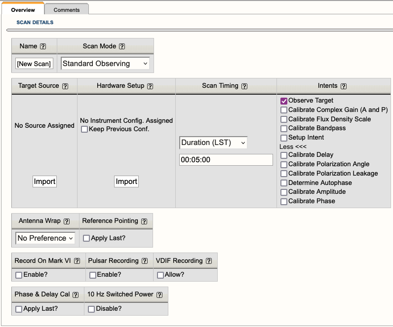 |
| Figure 4.3.6: New Standard Observing (STD) scan showing all available parameters and intents. |
|
Scan Parameters |
|
|---|---|
| Name |
Name the scan something useful to help keep organized while building the observation. Note, if you import a source before naming the scan, the scan will inherit the name of the source. You may change the name of the scan at any time. |
| Scan Mode |
Standard Observing (STD): The most commonly used mode for science targets and calibrators (e.g., complex gain (amplitude and phase), flux density scale, bandpass, delay, etc.). Interferometric Pointing (IP): Generally used in high frequency (> 15 GHz) observations to improve telescope pointing. Tipping (TIP): For measuring opacity curves. Currently not in use. Holography (H): For measuring antenna response. Internal NRAO use only. On The Fly Mosaicking (OTFM): For taking data in a constant slew that is different from compensating for Earth rotation. Solar (SOL): For a science target that is located near or on the solar disk. When a scan mode is selected, some of the scan parameters will change and the abbreviation will change in the SB scan list on the left-hand column. For a more detailed overview of the scan modes, refer to the Scan Modes in Detail section. |
| Target Source |
To select the source you wish to observe (i.e., science target or calibrator), click on the Import button, choose a Source Catalog (or Source Group within that catalog) and click on the Change button. This component pulls directly from the SCT. Any changes made to a source position within the SCT, the source must then be re-imported into the SB. New for 1.31 is the ability to filter the search across multiple source catalogs. See below in OPT 1.31 User Interface Update. |
| Hardware Setup |
To select the resource you wish to use, click on the Import button, choose a Resource Catalog (or Resource Group within that catalog) and click on the Change button. This component pulls directly from the RCT. For any changes made to a resource within the RCT, the resource must then be re-imported into the SB. New for 1.31 is the ability to filter the search across multiple resource catalogs. See below in OPT 1.31 User Interface Update. Special Notes:
|
| Scan Timing |
The scan timing determines the length of the scan. Duration(LST) is the default and the only valid option. The 5 min duration is also a default value but should be adjusted as needed. The duration of a scan includes the time it takes for the antennas to slew to the source plus the time spent on the source, i.e., slew + on source time = duration. Using the Duration(LST) scan timing mode will keep the length of the SB static. This in turn makes dynamic scheduling feasible. The OPT assumes a 20 second duration at the start of a scan to allow for receiver setup and changes in the focus and rotation of the subreflector. For observations that are switching between P-band and L-band, or P-band and S-band, more time is needed to account for the subreflector changing position. Please review the Exposure and Overhead section of the Guide to Proposing. It is possible to create SBs in On Source(LST) to investigate slew times between sources, etc., but the SB must be converted to Duration(LST) prior to submitting. This can be done best by selecting a viable LST start time in the Reports page, clicking Update to recalculate the slew times, and to make use of EDIT → TO DURATIONS from the top menu. |
| Intents |
The default is Observe Target, however it is very important to select the correct scan intent(s) for the corresponding sources. For example, the first scan for all SBs must use the Setup Intent (and no other intents). The setup intent tells the executor to set the attenuator levels on the antennas for the duration of the observation. Alternatively, the science target scans should only use the Observe Target intent and calibrators should only use their corresponding calibrator intent(s), i.e., calibrate complex gain (A and P), calibrate flux density scale, calibrate bandpass, etc.. For the calibrators, more than one scan intent may be selected. Do not use the Observe Target or Setup Intent on the calibrator scans. Note, do not use the Determine Autophase scan intent. This is only for phased VLA observations. |
| Antenna Wrap |
No Preference: The antennas will have no instructions on which direction to begin moving in AZ. CW (right): The antennas will be instructed to move clockwise in AZ. CCW (left): The antennas will be instructed to move counterclockwise in AZ. How and when to use antenna wraps is explained in the Antenna Wraps section of the Observing Guide. |
|
Reference Pointing Apply Last? |
This can only be selected on scans which are preceded by a scan using the Interferometric Pointing mode. Selecting this option on a scan will apply the pointing corrections during the observation. Note, pointing corrections cannot be applied after the observation has been taken. Therefore, it is crucial to correctly set this up in the SB. |
|
Over the Top Allow? |
This setting is still being tested and should not be selected. More details can be found under the Tipping (TIP) section. |
|
Record on Mark VI Enable? |
This setting is only used for phased VLA observations (VLBI). |
|
Pulsar Recording Enable? |
For phased-array pulsar observing only, enable this setting in order to record pulsar data for this scan. |
|
VDIF Recording Allow? |
This is only used for eLWA and radar observations. |
|
Phase & Delay Cal Apply Last? |
This setting is used for phased VLA observations (VLBI or pulsar) and should not be selected otherwise. |
|
10 Hz Switched Power Disable |
This setting disables the 10 Hz switched power calibration signal for this scan. During pulsar-mode observations the switched power should usually be disabled during pulsar scans and enabled during calibration scans. Otherwise this setting should not be used. |
| Comments tab |
You may add personal notes within the text box in the comments tab. |
Adding Scans
There are two methods for adding scans, either create a new scan or copy and paste an existing scan anywhere in the list of scans.
Add a new scan:
Select the scan you wish to add a new scan before or after.
- FILE → CREATE NEW → SCAN → BEFORE
- This will add a new scan before the scan you selected.
- FILE → CREATE NEW → SCAN → AFTER
- This will add a new scan after the scan you selected.
- FILE → CREATE NEW → SCAN → IN
- This will add a new scan in the selected SB or a selected loop. (Scan loops will be explained in the next section.)
Copy/paste a scan:
Select the scan you wish to copy.
- EDIT → COPY <name of scan>
- EDIT → PASTE BEFORE <name of scan>
- This will paste the scan before the scan you have selected or before the loop you have selected. (Scan loops will be explained in the next section.)
- EDIT → PASTE INTO <name of scan>
- This will paste the scan into a selected loop.
- EDIT → PASTE AFTER <name of scan>
- This will paste the scan after the scan you have selected or after the loop you have selected.
You may also use the copy and paste
icons located in the icon menu. The paste icon option will only paste the scan after the scan you have selected.
Scan Loops
To create a scan loop, select the scan you wish to either create the loop before or after and select,
FILE → CREATE NEW → SCAN LOOP → BEFORE (or AFTER)
Once a loop has been created, you can create new scans within the loop, copy/paste scans into the loop, and create more loops within the loop.
Scan loops are useful for creating a repetition of scans, i.e., for phase referencing (complex gain calibrator scan plus science target scan(s)). Loops can be named, be given many iterations, and contain a useful feature called Bracketed. If the Bracketed option is selected it will perform your first scan within the loop one extra time at the end of the loop.
Figure 4.3.7 shows four examples of bracketing the science target with the complex gain calibrator.
| No Loop | Normal Loop | Bracketed Loop | |
|---|---|---|---|
| individual Scans | two different orderings | should start with calibrator | |
| Figure 4.3.7: Four different bracketing styles. In these examples, Cal is an abbreviation for complex gain calibrator. | |||
Bracketing Options
- No Loop: This option does not utilize scan loops, however it is a valid option for bracketing the science target with the calibrator.
- Normal Loop: Two options are represented here.
- On the left, the calibrator is placed before the loop containing the science target and the calibrator.
- On the right, the calibrator is placed after the loop containing the science target and calibrator.
- Both options, the science target is appropriately bracketed by the calibrator.
- Bracketed Loop: The scan loop utilizing the bracket option is signified by two asterisks (**) next to the number of iterations the loop was assigned. With the bracket option selected, the first scan in the loop must be the calibrator scan so it will also be the last scan in the loop. This may not be apparent when only looking at the SB list of scans in the left-hand column, but will become more obvious when viewing the SB summary in the Reports tab.
A loop can contain any number of sources, not necessarily only a calibrator scan and a single science target scan. If your science target sources are near in the sky and you can use a single calibrator for all of the science targets, then you can group them in a loop with more than one, target scans before returning to your calibrator. Keep in mind that the total loop time should be shorter than the anticipated coherence time at our observing frequency. Loops may also contain loops. If your loop is selected, adding a new scan will place this new scan in the scan loop. The only difference with a normal scan is that this scan will be scheduled as many times as the "Loop iterations" specified, consecutively in a loop with the other sources in the loop. When finished with defining a loop, you may want to highlight it and then collapse it (using from the icon menu) for a more compact display in the tree.
Calibration
In addition to bracketing the science target(s) with its appropriate complex gain calibrator, it's important to understand when and where to add interferometric pointing (reference pointing) scans for high frequency (> 15 GHz) observations, where to place the flux density scale calibrator or bandpass calibrator (beginning, middle, or end of the SB). The Observing Guide has specific sections to help guide you on how to setup a high frequency or low frequency observation. However, the placement of some calibrators, i.e., flux density scale calibrator, will be determined by where that source is in the sky relative to the science target(s). Is it rising or setting? Double check the EL curve of the sources in the SCT (under the Images tab of a source) to help determine a good placement of the flux density scale calibrator. The placement of the flux density scale calibrator will also restrict the LST start range. There are many important factors to consider when creating an SB.
Below is a listing of specific sections within the Observing Guide helpful for setting up observations:
The Observing Guide also contains sections on Spectral Line, Polarimetry, Subarrays, Mosaicking and OTF, Moving Objects, VLBI at the VLA, and Pulsars under the Commonly Used Observing Modes section.
If at any time you are unsure of what to do or where to start with creating your SBs, please do not hesitate to contact us through the NRAO Science Helpdesk.
Filter in Import Search
Filter Source Search
Users can filter their source search in a source catalog from within the OPT. This can be useful if the source catalog in question has many source entries, such as sources used for a survey. Figure 4.3.8 shows how to activate the Filter search. Figure 4.3.9 shows the parameters available for the Filter.
Figure 4.3.9 explained:
- Source Catalog: the catalog upon which you wish to search
- Source Group: if you have groups in your catalog, you can search them individually or all of them
- Sources - Stop Filter: this will collapse the Filter options
- Name: filter by name of source
- RA: filter by RA position - Reset button resets RA to 0h 00m 0.00s (Note: when entering values you must use units)
- Dec: filter by Dec position - Reset button resets Dec to 0d 00' 0.00" (Note: when entering values you must use units
- Radius (deg): search radius in degrees based upon RA and/or Dec position - Reset button resets Radius to 1.0d
This same filter functionality is also available in the Bulk Scan Edit tab.
| Figure 4.3.8: Activating the Search Filter | Figure 4.3.9: Search filter options |
Filter Resource Search
Users can filter their resource search in a resource catalog within the OPT. This can be useful if the resource catalog in question has many resources. Figure 4.3.10 shows how to activate the Filter search. Figure 4.3.11 shows the parameters available for the Filter. Figure 4.3.12 shows what happens when you select a sampler that is not available for the receiver. Figure 4.3.13 shows that you can have multiple bands and/or samplers selected.
Figure 3.4.11 explained:
- Resource Catalog: the catalog upon which you wish to search
- Resource Group: if you have groups in your catalog, you can search them individually or all of them
- Resources - Stop Filter: this will collapse the Filter options
- Name: filter by name of source
- Filter Receiver Bands: filter by receiver band(s)
- Filter Sampler: filter by 3-bit and/or 8-bit samplers
The search results will appear as a list before the parameters section. Click on the button next to the source and select Change, or Cancel to quit.
This same filter functionality is also available in the Bulk Scan Edit tab.
| Figure 4.3.10: Activating the Search Filter | Figure 4.3.11: Search filter options |
| Figure 4.3.12: Incorrect sampler for receiver band | Figure 4.3.13: Example of multiband / sampler search results |


Connect with NRAO