Guide to Proposing for the VLBA (and HSA/Global VLBI) Complete Manual
Obtaining Time on the VLBA
How to Propose
Observing time on the VLBA is available to all researchers, regardless of nationality or location of institution. However, only 50% of the operational time on the VLBA is available for “open skies” observing. The other 50% is allocated for use by the US Naval Observatory. The allocation of open skies observing time on the VLBA is based upon the submission of a VLBA Observing Proposal using the online Proposal Submission Tool (PST) available via the NRAO Interactive Service web page, at my.nrao.edu. The online tool allows the user to assemble a proposal by specifying the requested observations using online forms, and uploading the required scientific justification. More specific info on using the online tool, and policies related to proposal types, scientific justification page limits, etc., can be found in the NRAO User Portal and Proposal Submission Guide. VLBA-specific details, including capabilities offered for the next proposal deadline, can be found in the current Call for Proposals and the VLBA Observational Status Summary (OSS). For a brief overview of the VLBA, please see the Introduction to the VLBA.
In addition to the general capabilities outlined in the Call for Proposals and the OSS, NRAO offers a VLBA Resident Shared Risk Observing (RSRO) program for those who would like to push the capabilities of the instrument beyond those offered for general use. Details about RSRO projects are available on the web in the VLBA OSS - Offered Capabilites page.
It is also possible to obtain VLBA observing time by proposing to NASA missions, under cooperation agreements established between NRAO and those missions. Such programs exist for the XMM-Newton, Chandra, Fermi, Swift and HST missions. Astronomers interested in those joint programs should consult the relevant mission proposal calls for more information.
Note that it is possible to search cover sheets of proposals previously approved for time since semester 2005C using the Proposal Finder Tool (PFT).
The actual VLBA proposal process consists of the following steps:
- Develop rationale: Before writing a proposal, the proposer must develop the scientific rationale for the program, develop a source list, decide on the observing band(s) to be used, and estimate the expected source strengths and their detectability. For spectral-line sources, the proposer also must decide on the desired velocity resolution, and convert that to a spectral resolution.
- Create Proposal in the Proposal Submission Tool (PST): After logging into NRAO Interactive Services, click on "Proposals" and then "New Proposal" on the top to the far right of the screen. Then click on VLBA/HSA and "Create" (again on top to the far left). A proposal template will be created for you; click on the proposal number and this will open the proposal for you. There are seven screens to choose from and edit (there is an additional screen where you can find your disposition letter after the proposal has been reviewed).
- General: Title, abstract, proposal type, etc.. Edit this page by clicking on the "edit" button to top to the far right.
- Authors: List of authors and contact information. You can add an author by clicking on the "Add" button to the right on the page. Then search for your co-authors and if they are not in the database you can add them.
- Scientific Justification: Upload a pdf or txt of your scientific justification, no more than 4 pages in length for a Regular or Triggered proposal (including figures, tables and references) with an 11pt font. Large proposals (200 hours or more) are limited to 6 pages with 11pt font. Director's Discretionary Time (DDT) proposals are limited to 2 pages with 11pt font.
- Technical Justification: An important part of the proposal to be submitted is the Technical Justification. Previously merely a required section in the Scientific Justification, it is now a separate element of each proposal. Instead of the free format used in the Scientific Justification, we ask proposers to supply information on a number of standard topics, covering the wide range of technical issues of importance. We have found that this reduces the likelihood that information is left out needed by the Technical Reviewers to judge the feasibility of the project as proposed. Follow the links in the form to obtain more information on the individual topics. Click here to see an example. Note that with technical information contained on this page space is freed up in the Science Justification.
- Sources: List of sources. One slightly confusing thing here is that you have to create a "New Source Group" to add sources (button on upper right). After creating a group you can either add sources to it by hand or search for them with NED/SIMBAD. Adding sources to this section does not mean any time has been requested for them, they must be linked to a telescope resource in Sessions. Except for proposals where the sources are not known a priori (e.g. triggered proposals), all target sources must be included in the source list. Calibrators may also be added to this list, but it is not required.
- Resources: Resources requested from the VLBA (antennas, frequencies, bit rates, correlator, etc.). To add a resource click "add" on the right. If proposing for the VLBA/HSA then the "Socorro-DiFX" correlator should be used. Set which telescopes are being requested and then set the "Observing Parameters" and "Correlation Parameters" based on the scientific goals of the project. For most continuum experiments you will want the highest sustainable aggregate bit rate (currently 4 Gbps; see the relevant section of the OSS), i.e., the largest bandwidth and therefore the highest sensitivity. For spectral line observations choose the number of baseband channels and their widths based on the expected frequency coverage of the lines, leaving some continuum on either side available for calibration. If bandwidths narrower than 1 MHz are required, see the spectral resolution section of the OSS.
- Sessions: Describes the amount of time requested, and how it should be divided among the various sources and resources. Click on "New Session", this is where you actually request time on your sources at different frequencies.
- Examine and Submit: Go back to "My Proposals" and click on the printer icon (looks like a printer) next to the proposal code to see what the proposal will look like to a reviewer. Once you are satisfied click the submit (large arrow) button to submit the proposal.
Students
Students planning to use the VLBA for their Ph.D. dissertation must submit a Plan of Dissertation Research of no more than 1000 words with their first proposal. This plan can be referred to in later proposals. At a minimum, the plan should contain a thesis time line and an estimate of the level of VLBA resources needed. The plan provides some assurance against a dissertation being impaired by an adverse review of a proposal when the full scope of the thesis is not seen. The plan can be submitted via NRAO Interactive Services. Also see the Student Proposals and Dissertation Plans section of the NRAO/GBO Users' Policy Manual for more details. Students are reminded to submit their plan comfortably in advance of the proposal deadline. New thesis plans must be in PDF format to enable science reviewers to easily access the plans. Students who have not yet graduated, but have active plans on file, should consider updating those plans to a PDF format if they are not already in that form.
Timeline
Time on the VLBA is scheduled on a 6-month semester basis. Semester A observations typically take place February through July and have a proposal deadline on the Wednesday closest to August 1 in the previous year; Semester B observations take place from August through January and have a deadline on the Wednesday closest to February 1. The call for proposals typically goes out 3–4 weeks prior to the deadline.
For details on the evaluation of submitted proposals we refer to the NRAO Proposal Evaluation/Time Allocation page. Because of competition, even highly ranked proposals are not guaranteed to receive observing time. Observing time at each VLBA station will also continue to be limited by ongoing testing and maintenance activities; for more information, see the section on Scheduling Considerations in this document.
The Proposal Review Process
Determining who gets time on the VLBA (and VLA, GBT, etc.) involves 6 steps.
- Proposal submission: people who wish to use the instruments request time.
- Technical review: NRAO scientists and analysts read the Technical Justification (TJ) section of each submitted proposal to determine whether or not the proposed projects are feasible, need adjustments, or are impossible to successfully observe. The science objectives are only considered as they pertain to the requested observations, not their scientific merit.
- Scientific review: Science Review Panels (SRPs), made up of experts outside of NRAO, review each proposal for scientific merit. All the proposals that are considered by a SRP are then ranked.
- Time allocation: the Time Allocation Committee (TAC) combines the ranking with the technical reviews to determine which projects are granted observing time, how much time, and at what priority.
- Director's review: The observatory Directors, Chief Scientists, the NRAO Assistant Director for Science Support and Research, and other observatory staff review the results from the SRP and TAC to ensure that all NRAO procedures and policies have been followed. This review may result in some adjustments to priorities.
- Disposition letters sent and the TAC report is published: Proposers learn the results of the review process. The goal is to send the disposition letters at least 2 months before the next deadline.
The entire process, from submitting your proposal to receiving the disposition letter, typically takes between 3 and 4 months.
Director's Discretionary Time
It is also possible to propose for Director's Discretionary Time (DDT). DDT is reserved for Targets of Opportunity and for Exploratory Time. DDT proposals may be submitted at any time with the understanding that they should only request for semesters for which the proposal deadline has passed. The DDT proposals must be submitted through the PST. DDT proposals are reviewed by the DDT review committee the basis of the proposals' scientific merit, conflict status, LST pressure, and technical feasibility.
NOTE: The Science Justification for a DDT proposal is limited to two (2) pages.
A Note on VLBA Observing Semesters
The VLBA observing semesters are always the same. VLBA Semester A begins February 01 and ends July 31; VLBA Semester B begins August 01 and ends January 31. Therefore, VLBA observing semesters may not always align with the VLA observing semesters, which vary based on array configuration.
Joint VLBA/VLA/GBT Proposals
Observing programs that require combinations of the VLBA, GBT, and/or the VLA should submit a proposal for each of the requested telescopes, with a clear justification for each, as has been the case to date. The proposals will be reviewed and considered jointly by the Time Allocation Committee. VLBI proposals which request the GBT or VLA (or any other HSA telescope) as elements of the VLBI array do not need separate proposals---those telescopes can be selected as separate VLBI stations from a VLBA/HSA proposal.
For example, a program to monitor a transient source with the VLA and get occasional VLBA observations to look for non-thermal components would need to submit identical proposals to both the VLA and VLBA.
Array Options
Standard VLBA
The standard VLBA includes 10 identical 25-meter antennas located at sites across the United States:
- Saint Croix (SC) in The US Virgin Islands
- Hancock (HN) in New Hampshire
- North liberty (NL) in Iowa
- Fort Davis (FD) in Texas
- Los Alamos (LA) in New Mexico
- Pie Town (PT) in New Mexico (the closest VLBA site to the VLA)
- Kitt Peak (KP) in Arizona
- Owens Valley (OV) in California
- Brewster (BR) in Washington
- Mauna Kea (MK) in Hawaii
For live webcam images of the VLBA sites, visit the VLBA Virtual Tour.
For additional information on the VLBA sites, see the VLBA Observational Status Summary (OSS).
VLBA + Single Dish VLA (Y1)
A single dish VLA antenna (Y1) can be used in conjunction with the VLBA. The inclusion of such a dish would provide a short (~50 km) baseline to the VLBA station at Pie Town (PT).
VLBA + Three VLA Antennas (Y3)
This document describes the particular case of three VLA antennas (Y3) being used in conjunction with the VLBA‡, with each of them correlated with the VLBA antennas and among themselves. This VLBA + Y3 mode has been commissioned through RSRO projects.
The intention of Y3 in the context of this document is to provide VLBI with additional short spacings when combined with the VLBA. However, the use of Y3 limits the bandwidth on the VLA antennas. Relative to Y1, Y3 has 3 times the collecting area but only half the bandwidth due to recording-data-rate restrictions. Therefore, while it adds multiple baselines and enhances the uv coverage, in terms of sensitivity, for continuum observations, Y3 is roughly equivalent to adding another single antenna (i.e., in terms of sensitivity Y3 is roughly equivalent to 2 VLA antennas).
For proposals requesting Y3, we note that:
- Y3 is only available for the VLA's A-configuration when the outer antenna baselines are useful when combined with the VLBA.
- Proposals must clearly demonstrate why single VLA antenna (Y1) is insufficient for the science proposed, because Y3 projects require significantly more resources than Y1. Note that Y3 does not appreciably increase the sensitivity for continuum observations over Y1 because of the bandwidth limits on Y3 noted above.
- If there are no restrictions on scheduling and the full VLA is not required for the project then Y3 will be observed in the moves from from BnA (or B) to A and from A to D configurations when the outer antennas are at their A-config locations.
- If a Y3 project must be observed during full A configuration, e.g., the project is triggered, then proposals are strongly encouraged to also include a proposal for how to use the remaining VLA antennas in a regular (non-phased) VLA mode to support the proposed VLBA+Y3 science. These should be submitted as joint VLBA/VLA proposals, with the VLBA proposal including the Y3 and the VLA proposal for the remaining 24 antennas. Because most VLA proposals for A-configuration require the full resolution of the array there will, in general, be very few other projects that can be carried out with the 24 VLA antennas not being used for the Y3 experiment, therefore proposals that do not include a request for the remaining 24 VLA antennas must have a very strong justification for not using the entire array. Note again, that if the project can be scheduled in the moves between configurations this is not required.
- Pointing modes are not available with Y3. VLA single-dish blind pointing is generally not as good as VLBA blind pointing, so there is a risk the VLA antennas may be slightly off-source. This will have a greater impact at higher frequencies.
‡There is another Y3 concept that has not yet been tested nor commissioned and we note it here for completeness. This mode can be proposed under RSRO. In this other mode, known as Y3-IP, three VLA antennas are used to enable interferometric reference pointing (IP) on the three VLA antennas when observing at high frequencies (> 15 GHz) along with the VLBA. During the observing session, when not doing IP: a) the three antennas can be phased up, summed, and recorded as a single VLBI element, giving approximately three times the sensitivity of a single VLA antenna, or b) the data from one of them can be recorded for VLBI if a wide field of view is critical for the science. Since this does not need to use the ends of the arms, in fact short baselines would be preferred, this type of Y3 does not include the restrictions detailed above.
High Sensitivity Array (HSA)
High Sensitivity Array
For projects that require the maximum sensitivity, users should consider submitting proposals for the High Sensitivity Array (HSA). Currently, users may add the following telescopes to the VLBA to improve sensitivity:
- Effelsberg: Effelsberg has often been used in conjunction with the VLBA, and is frequency agile at 5 GHz and above. For more information about including Effelsberg with the HSA we refer to the Effelsberg HSA page and the Effelsberg VLBI page.
- Green Bank Telescope: The Green Bank Telescope is also commonly used with the VLBA, and is frequency agile (with some limitations) at all its bands. See the VLBI at the GBT page for more information.
- Very Large Array: The Very Large Array (VLA) is available in phased-array mode (Y27). Please see the VLBI at the VLA, and the HSA/GMVA/Global VLBI and Building a Schedule chapters of the Guide to Observing with the VLBA pages for further considerations.
Check the OSS for any limitations or special instructions for each HSA telescope. Also, make sure to use the EVN sensitivity Calculator to estimate the rms noise for your observation.
Important note on possible HSA expansion: After the loss of the 305-m Arecibo radio telescope, the NRAO has looked into the possibility of having other radio telescopes be part of the HSA. Considering that there are currently no agreements to include other stations, the HSA continues to be the addition of the GBT, the phased VLA, and/or Effelsberg to the VLBA in the semester 2022A.
Special considerations for HSA proposing and observing
- Proposals: Proposals should be sent to NRAO only, through the Proposal Submission Tool, which can be accessed via NRAO Interactive Services. Click on VLBA/HSA when creating the proposal.
- Field of View: The field of view of the HSA is more limited than for the VLBA, because of the smaller primary beams of all the HSA telescopes, especially the phased VLA (Y27). For the latter, note that the larger the extent of the array, the smaller its field of view.
- Scheduling: Use NRAO's SCHED software to make the observing schedule, available from anonymous ftp at: ftp.aoc.nrao.edu The SCHED manual has several example files to get you started. Please be sure to use the latest version of the software, or to run SCHED on the final schedule file submission.
For scheduling note that:- Effelsberg has station name 'EB_VLBA'
- GBT has station name 'GBT_VLBA'
- The phased VLA has station name 'VLA27'
- Slew speeds:The Effelsberg, GBT, and VLA slew speeds are slower than for VLBA antennas. The GBT slew rate also decreases during cold weather. Be aware of this when writing your schedule, and be sure to examine the output from SCHED. SCHED has the latest information on slew speeds, including acceleration and deceleration, for all telescopes.
- Pointing: Since the Effelsberg and GBT antenna beamwidth is ~4 times smaller than those of VLBA antennas, periodic pointing checks are essential, especially during short wavelength observations. Observers should leave frequent gaps in their VLBI schedules (~10 mins each) to allow the telescope operators to make these checks. They should be about every hour or two at 4cm, and more frequently at shorter wavelengths. See the VLBI on the GBT page for more specific information on how and when to schedule pointing checks.
The VLA also requires pointing at frequencies lower than the VLBA, for the VLA however the pointing must be scheduled by the observer in SCHED. See VLBI @ the VLA:Scheduling Hints for examples more information. - Submitting Schedules: The submission deadline is two weeks before the observation. The input file for SCHED, incorporating any non-standard setup files, should be e-mailed to vlbiobs@nrao.edu. If you have problems with your schedule contact vlbiobs@nrao.edu. If any changes are made to schedule after the deadline the support personal at all the telescopes must be contacted.
- For the VLBA and the phased VLA notify vlbiobs.
- For the GBT notify Pedro Salas and Toney Minter.
- For Effelsberg notify the Observing Friend.
- Frequencies: While the GBT has frequency coverage equal to the VLBA, changing receiver bands takes 5-10 minutes. For more details on changing frequencies at GBT see the VLBI on the GBT page.
The VLA and VLBA have similar frequency bands, but the VLA receivers generally have a wider tuning range.
See Instructions for Joint VLBA + Effelsberg Observing for information about frequency availability and changing between frequencies at Effelsberg. - Non-Standard Frequency Setups: Observers using non-standard frequency set-up files (i.e. not one supplied with the current version of SCHED) should contact the technical friends at the telescopes. These are Pedro Salas at the GBT and Uwe Bach at Effelsberg. Contact should be made well before the observations so that any special files needed for tuning can be made in good time.
- Correlator: All observations will be correlated at the VLBA correlator in Socorro.
- Archive: All observations will be archived on-line and password protected during the 1 year proprietary period. Request a project access key from the data analysts. See the NRAO data policy for further details.
Global VLBI
Global VLBI
Users interested in the maximum possible angular resolution, or extremely long observations in a single track, should consider submitting a Global VLBI proposal. Global VLBI falls into two categories:
- Global 3mm VLBI (GMVA)
- Global cm VLBI
NOTE: submissions by email, fax, or paper will not be considered for any Global VLBI opportunity.
GMVA
GMVA projects are correlated at the Max Planck Institute for Radio Astronomy in Bonn, Germany. Users interested in GMVA should submit proposals via the NRAO Proposal Submission Tool (PST) at the usual VLA/VLBA deadline: The Wednesday closest to February 1 and August 1 by 1700 Eastern Time. New users are strongly encouraged to contact the VLBA and/or GMVA staff to get assistance in preparing their proposal.
Global cm VLBI
Global cm VLBI involves combining the VLBA with the European VLBI Network (EVN). Proposals for Global cm VLBI must be prepared and submitted using the EVN NorthStar Tool. The EVN Northstar tool will automatically send copies of Global cm VLBI proposals to NRAO for assessment. Submission deadlines for Global cm VLBI do NOT follow the normal NRAO schedule. Instead, the proposal submission deadlines are are February 1, June 1, and October 1 by 23:59:59 UT. Additional guidelines for EVN and Global cm VLBI can be found at the EVN Guidelines for Proposal Submission and the Using the EVN website.
Scheduling Considerations
Sessions
When the submitting a proposal for either VLA or VLBA observing time, you must enter the observations you plan in the form of “sessions” in the Proposal Submission Tool (PST). Each session is a unit of observing time (target + resource + time) which will be considered by the Time Allocation Committee (TAC) when determining how much time to grant a proposal. If your sessions are not properly set up in the PST, it can strongly impact the TAC’s decisions when assigning observing priority. Users are encouraged to consult the guidelines for creating sessions for the VLA. Most of these guidelines are also relevant for creating VLBA sessions. One major difference between VLA and VLBA is that VLA sessions require you to enter a Local Sidereal Time (LST) range for each, while VLBA sessions require a Greenwich Sidereal Time (GST) range. Also unlike the VLA, the PST does not calculate the GST range for a session; instead, proposers should calculate this using SCHED or the EVN PlanObs or some other tool. For more details on LST and GST, including a tool to convert between GST and LST, check out the US Naval Observatory's Sidereal Time page.
Proposers are strongly encouraged to create “dummy” observing schedules with the SCHED software. This will ensure that you properly account for considerations such as slew time, rise/set times, and calibrator scans. Keep in mind that you may need scans on bandpass calibrators, fringe finders, polarization calibrators, and phase reference sources. This is covered in more detail in the Exposure and Overhead chapter.
High Frequency Observations
High frequency observations are susceptible to atmospheric effects, such as air turbulence and water vapor. During the summer months, and especially during daytime, conditions appropriate for high frequency observing are limited. Other limitations may include needing night-time observing or observing during dry seasons for increased phase stability. With the stricter weather constraints on high frequency (> 12 GHz) observations, programs are in competition for less available time.
If your science requires high frequency observations, it may be best to propose for a semester when your target will be up at night. However, this is not always possible, especially considering that not all VLBA stations will experience night and day at the same time. Therefore, proposers are strongly encouraged to carefully consider which observing frequencies are absolutely necessary for their science during a particular semester. If a proposal requires large amounts of daytime high frequency observations it may be extremely difficult to schedule successfully. In such a a case, the TAC may allot a reduced number of hours or determine the project is unfeasible even if the proposal was highly ranked by the Science Review Panel (SRP).
Low Frequency Observations
Radio frequency interference (RFI) from terrestrial sources is not as large a concern for VLBA observing as it is for VLA or single-dish observing. While terrestrial RFI does impact low frequency observations more than high frequency observations, the VLBA antennas are located so far apart that the RFI does not (usually) correlate between baselines. However, RFI is becoming more ubiquitous at low frequencies and similar RFI may be present at multiple antennas despite their geographic separation. Strong RFI at a single antenna can still lead to reduced sensitivity (since the VLBA only has 10 antennas compared to the VLA’s 27). Some satellite transmissions can lead to catastrophic loss of data across all (or nearly all) VLBA antennas, but such occurrences are relatively rare and tend to happen in the dedicated transmission bands. However, the number of satellites is growing at high rate and users who are planning long-term projects are encouraged to take this into consideration when designing their observing plans.
Low frequency observations on the VLBA are affected by ionospheric variations more than on the VLA. Because the VLBA antennas are so spread out, the ionosphere needs to be measured above each individual station. While the Total Electron Content (TEC) measurements are made, using them is not 100% effective in nullifying phase issues the ionosphere creates in low frequency VLBI data. If your science requires that the phases be as perfectly calibrated as possible at lower frequencies, you may need to use 13/4-cm dichroic system for some observations in addition to your science band(s) in order to accurately measure the effects of the ionosphere on your observations. See VLBA Scientific Memo 23 for more details on this issue.
Low Declination Sources
Unlike the VLA, the VLBA does not have a single declination limit. Instead, each station has its own limits. See the VLBA Declination Limits section of the VLBA OSS for details on the limits for each station.
In general, NRAO recommends that a you observe a source when it will have an elevation above about 20 degrees at each participating station. This helps make calibration easier. However, depending on your science, you can try observing at lower elevations. An elevation of 10 degrees is the practical limit for most stations. Below 10 degrees, you will be more likely to encounter “spill-over” (signal reflected from or originating from the ground) at lower frequencies (<4 GHz), and you will need to deal with a large amount of atmosphere at higher frequencies (>10 GHz). Also, keep in mind that RFI tends to increase as the telescopes point to lower elevations because they will be more likely to look at man-made objects (cell phone towers, cars on nearby roads, etc.).
If you are observing at very low frequencies (< 1 GHz) or very high frequencies (>40 GHz), the practical elevation limit for each station is closer to about 20 degrees.
Your science goals, your observing frequency, and the nature of your target will determine how low you are willing to observe a source. For example, if you are planning to observe a very bright source at X-band (4cm, ~8 GHz), it may be possible to observe it all the way down to the horizon limits of the stations. However, if you are doing a phase-referenced observation at Q-band (7mm, ~42 GHz), it would be in your best interest to only observe the sources when they have elevations of 20 degrees or higher.
If you have a low-declination source that you would like to observe with the VLBA, it is a very good idea to make sure it will be visible for long enough and at enough antennas to achieve your goals. A good tool to use for this is the JIVE planobs tool. This tool allows you to plot the elevation of a source as a function of time at each antenna site for many VLBI arrays (VLBA, EVN, LBA, etc.).
To use the JIVE planobs tool to plot the elevation of a source at each of the VLBA stations, follow these steps:
- Select "Manual Mode"
- Select your observing band from the drop-down menu
- Select "Find epoch for given source"
- Enter the source coordinates
- In the “Select default VLBI Network(s)” drop-down menu, select “VBLA: Very Long Baseline Array”, and add a check in any additional stations you will use if you plan on proposing for Y1, HSA, or Global VLBI
- Optionally, you can also specify the percent of time on target, the data rate, and the setup details (the tool is also useful for estimating sensitivity and resolution, if you want to calculate those as well; see the Exposure and Overhead chapter)
- Click "Compute Observation" (near the top left of the page)
- After the program is done computing, click on the "Elevations" tab to see the plot of elevation vs. time and the plot of when a source is visible from each station.
Note that the JIVE planobs tool uses 10 degrees elevation as a hard cutoff for when a source is visible from each station.
Another method to estimate the amount of time a source spends above a certain elevation at each station is to build a SCHED .key file for the observation. Then, you can run SCHED and look in the .sum file or use the SCHED plotting tools, especially the “uptime” plot, to get information on the source elevation at each station for each scan. SCHED has information about the horizon limits of each station (in the catalogs/stations_RDBE.dat file), so it does a good job of estimating when a source will be visible at each station.
In addition to the effects on sensitivity and the ease of calibration, it is good to keep in mind that the uv-coverage will be worse when observing low-declination sources. If your science goals include high dynamic range imaging of complex structures, uv-coverage may be a bigger concern than sensitivity. The JIVE planobs tool and the SCHED plotting tools can both generate plots of the estimated uv-coverage for an observation.
Other Special Considerations
There are several other considerations that may impact you observation.
Coordinated Observations
In the event that you need simultaneous observations with the VLBA and another instrument (e.g., you need to know the ratio of flux density from compact components to total flux density), you will need to consider the scheduling constraints of both telescopes. Typically, it is recommended that you schedule both observations as “fixed date” observations to avoid any uncertainties in observation times that may be introduced by the dynamic scheduler.
Moving Objects
While the VLBA is capable of observing objects moving with respect to the celestial coordinate system (e.g., asteroids, planets, etc.), it is not a default mode. Special scheduling techniques are required. If your science target is such an object, you are encouraged to contact the VLBA staff to consult on an observing strategy. Also, be aware that your object may be in the “near field” and require special techniques for calibration and imaging.
Sun Avoidance
Observations of objects close to the Sun can have extra difficulties in calibration due to increased phase fluctuations and elevated system temperatures. Unless your science specifically requires pointing at an object near the sun (e.g., testing the effects of General Relativity on the astrometric position of a background quasar), it is strongly recommended that you avoid observing near the Sun. The lower the observing frequency, the further from the Sun you should point. The following table contains the recommended minimum angular distance from the Sun to avoid amplitude reduction on the longest VLBA baselines for select observing frequencies:
| Freq. | Ang. Separation |
|---|---|
| 327 MHz | 117. deg |
| 610 MHz | 81. deg |
| 1.6 GHz | 45. deg |
| 2.3 GHz | 36. deg |
| 5.0 GHz | 23. deg |
| 8.4 GHz | 17. deg |
| 15.0 GHz | 12. deg |
| 22.0 GHz | 9. deg |
| 43.0 GHz | 6. deg |
NOTE: The VLBA scheduling software, SCHED, will warn you if your observations are closer to the Sun than recommended.
Daily UT1-UTC Observations
The VLBA makes daily observations to measure the Earth orientation parameter UT1-UTC for the US Naval Observatory. These observations are centered between 1730 and 1930 UT, and last for no longer than two hours. Two antennas are used for these UT1-UTC observations (usually MK and HN). The necessary antennas may be temporarily removed from an ongoing science observation to complete the UT1-UTC scans. The VLBA Schedulers always attempt to minimize the impact of UT1-UTC scans on science observations.
Frequency Bands and Observing Systems
Frequency Bands
The VLBA antennas are equipped with 8 cryogenically cooled receivers and one UHF receiver. Together, they provide frequency coverage from 312 MHz to 90 GHz. The receiver bands and the System Equivalent Flux Density (SEFD) at a specified center frequency can be found in the VLBA Observational Status Summary (OSS).
The SEFD can be thought of as a sensitivity rating, where a lower SEFD means better sensitivity. Note that the lowest SEFD (best sensitivity) is in the 6 cm (C-band) receiver. The further the observing wavelength is from 6 cm, the worse the sensitivity gets. Consult the OSS for additional details about the receivers and their performance.
The VLBA also has a special 13/4-cm dichroic system that can observe at both 13 cm (S-band) and 4 cm (X-band) simultaneously. This mode is particularly useful for determining the impact of the ionosphere on observations, which can cause both Faraday rotation and dispersive delays in the data. If your science requires extremely well-calibrated phases at low frequencies or if you need the best possible precision in your polarimetry, you may want to supplement your observations with some 13/4-cm dichroic system observations on a bright calibrator to fully characterize the ionosphere.
Observing Systems
A Note on Terminology: The VLBA Observational Status Summary (OSS) now uses the term “data channel” to describe a subband with a single polarization. However, the Proposal Submission Tool (PST) still uses the term "baseband channels" and SCHED still uses the term “baseband converter” or “BBC”. To be consistent with the VLBA OSS, this document will use the newer terminology of “data channel”. Please keep in mind that “data channel” and “spectral channel” are NOT the same; each data channel is further divided into spectral channels.
The VLBA currently has two separate observing systems: The polyphase filterbank (PFB) and the digital downconverter (DDC).
PFB: The polyphase filterbank digital processing algorithm produces 16 fixed-bandwidth 32 MHz data channels within a single ROACH digital backend (RDBE). The total data rate is 2048 Mbps (2 Gbps).
DDC: the digital downconverter algorithm supports a wider range of bandwidths than the PFB system, with data channels as narrow as 1 MHz and as wide as 128 MHz. However, only 1, 2, 4, or 8 data channels are allowed. The total data rate can be as low as 4 Mbps or as high as 4096 Mbps (4 Gbps).
Choosing an observing system: The PFB has more data channels than the DDC, so it may be preferable when attempting to avoid specific narrow-band RFI. The ability to produce very narrow data channels with DDC make it better suited to spectroscopic observations. Users who require maximum sensitivity for continuum observations will also likely prefer the 4096 Mbps capability of the DDC system. Also, please note that while the DDC mode provides wider bandwidth and tuning flexibility, the PFB mode provides more accurate amplitude calibration and should be used if <10% flux density accuracy is required. You should carefully consider which system is the best match for your science goals.
Additional information on both observing systems can be found in the OSS in the Signal Processing chapter.
SCHED
Creating VLBA Schedules
The program observers will use to create VLBA schedules is called SCHED. Anyone who observes with the VLBA is required to submit their schedules as SCHED .key files. SCHED is also very useful for creating VLBA proposals. Proposers can use SCHED to determine when a source is visible at the various VLBA stations, and also create dummy schedules to estimate the total observing time needed for a project.
The instructions for installing SCHED can be found on the SCHED installation page. Users who require additional assistance with the installation can submit a helpdesk ticket. Once logged into the NRAO helpdesk, use the radio buttons to select “VLBA”, and then “VLBA Observing” (and be sure to specify that it is a SCHED issue in the subject line).
To determine when a source is visible to the VLBA stations, proposers can use the extremely simplified scheduling file uvcov.key. Proposers should change the sources in the file to their target sources. To get a summary of the times when each station can see each target, run SCHED on the .key file by typing
sched < uvcov.key
and SCHED will create a file called "uvcov.sum" in the current working directory with details about as when each source is visible to each VLBA station.
To see plots of the uv coverage, times above a minimum elevation, and elevation vs. time for the targets, type
sched
plot sch=uvcov.key
and SCHED will bring up a plotting GUI that will allow the user to create various figures. See the plotting section of the SCHED User Manual for more details on producing these plots.
Proposers are encouraged to create dummy .key files for their observations in order to determine their total observing time for their projects. If you are proposing for triggered Target of Opportunity (ToO) observations and do not know your target’s position, you can still create a dummy .key file with reasonable (or even worst-case) target coordinates just to estimate the total observing time for your project. SCHED comes packaged with a variety of example .key files to help new (and experienced) users get started. For a dummy schedule, it is not extremely important to have the exact setup you will use for your observations. What is important at the proposal stage is determining the amount of time your science targets are observable and estimating the total observation duration for each epoch. This is covered in more detail in the Exposure and Overhead chapter.
Once you have created your dummy .key, run SCHED by typing
sched < dummy.key
where “dummy.key” is the name of your dummy schedule file. This will generate several new files in your current working directory. The most important one at this point is the summary (.sum) file. The summary file contains a great deal of information about your schedule, including the total time on source for each target, the total run time of the observation, and when each antenna is on source.
4 Gbps Setups
The 4 Gbps observing mode on the VLBA is now operational. For more information on creating setups, including several examples of 4 Gbps setups, see Linford & Brisken (2020) and the "Building a Scheduling File in SCHED" chapter of the Guide to Observing with the VLBA. Some users who wish to create schedules using the 4 Gbps mode may need to contact NRAO staff to obtain assistance with creating the frequency setups in SCHED.
Correlator Setup including Multiple Phase Centers
The VLBA DiFX software correlator, developed at Swinburne University (Deller et al. 2007) and adapted to the VLBA by NRAO staff (Brisken 2008), offers great flexibility in correlating observed data. Details on the current version of the correlator can be found in Deller et al. 2011 and the DiFX Guide.
Spectral Channel Width
VLBA users may select the desired number of “spectral points” for their observations, keeping in mind the following:
- A maximum of 4096 spectral points per baseband channel is allowed for routine DiFX processing.
- A total of 132,096 points, summed over all baseband channels and polarization products, is all AIPS can handle.
- The minimum spectral channel width is 2 Hz. The number of spectral points in all baseband channels must be identical within each correlation pass, but different correlation passes may have different numbers of spectral points.
- DiFX also supports "spectral zooming", where users select a specific subset of spectral points to correlate. The location and width of these "zoom bands" must be communicated directly to the VLBA operations staff before correlation.
For more details on spectral channel settings, see the VLBA Observational Status Summary (OSS).
Integration Period
Users can specify nearly any correlator integration period they wish. However, individual integrations are quantized in multiples of the number of spectral points requested divided by the data channel bandwidth.
The default integration period is 2 seconds.
Multiple Correlator Passes and Multiple Phase Centers
The DiFX correlator allows users to perform multiple correlation passes on the observation data. Users must specify the number of correlator passes they need when defining their Resources in the Proposal Submission Tool (PST).
The DiFX correlator also allows for multiple phase centers to be specified per pointing. The current limit for the standard 10-element VLBA is about 600 phase centers at 2 Gbps (512 MHz polarization-summed bandwidth) for dual polarization. Two correlator passes may be required for 600 phase centers at 4 Gbps. Full polarization reduces the number of phase centers per correlator pass by a factor of 2. With multiple correlator passes, any number of phase centers may be achieved. For more information on the multiple phase center capability, see the OSS.
Users must specify the number of phase centers per pointing when defining their Resources in the PST. For a given Resource, use the "Number of Fields" item in to specify the maximum number of phase centers required for any antenna pointing. The requested spectral resolution and integration time should correspond to the desired initial number of spectral points per data channel (required to minimize bandwidth smearing) and the desired integration between u-v shifts (to minimize time smearing). A resulting expanded output data rate that exceeds the current limit, as well as any required multiple passes, must be justified specifically in the proposal.
Pulsar Gating
DiFX supports 3 time-based selection modes to facilitate pulsar observations:
- Binary Gating
- Matched-filter Gating
- Pulsar Binning
For more information on pulsar observing, see the OSS and Brisken & Deller (2010). Users who will require pulsar gating must select the “pulsar gate” option when defining their Resources, and describe their setup in the Technical Justification section of the proposal.
Calibration Considerations
A Note on Terminology: The VLBA Observational Status Summary (OSS) now uses the term “data channel” to describe a subband with a single polarization. However, the Proposal Submission Tool (PST) still uses the term "baseband channels" and SCHED still uses the term “baseband converter” or “BBC”. To be consistent with the VLBA OSS, this document will use the newer terminology of “data channel”. Please keep in mind that “data channel” and “spectral channel” are NOT the same; each data channel is further divided into spectral channels.
Flux Density Scale Calibration
Because the VLBA uses system temperatures and gain curves to determine the flux densities of targets, users are not required to schedule scans on flux density calibration sources.
Observations with the High Sensitivity Array (HSA; see Chapter 2.2) using the phased VLA should schedule time on a VLA absolute flux density scale calibrator (3C286, 3C138, or 3C147), although it is not required. Without a scan on one of these calibrators, user's will need to rely on the VLA's switched power for flux density scale calibrations, which is only good to about 10%. As additional benefit, the VLA flux density of all the sources can be independently determined and the observer can determine how much (if any) flux is resolved out on the long baselines.
For more details on VLBA flux density scale calibration, see the Amplitude Calibration section of the VLBA OSS.
Fringe Finding
In order to properly calibrate the phases and delays in your observation, you will need at least one scan on a bright (and preferably compact) target. In general, it is recommended that this scan last about 2 minutes. Users should chose a source that has strong signal on all baselines at their observing frequency. The NRAO maintains a list of recommended fringe finders. Considering the importance of the fringe finder scans to successful calibration, it is strongly recommended that user schedule these scans near the middle and/or end of the observation. Note that fringe finder sources can often also be used for bandpass calibration (see below).
If an observation lasts longer than about 4 hours, it is recommended to observe a fringe finder at least twice (if the fringe finder is also the bandpass calibrator, the same fringe finder should be observed both times).
Bandpass Calibration
In order to properly calibrate the bandpasses for each data channel, you will need at least one scan on a bright target. This can often be the same target as the fringe finder.
Self Calibration
Bright VLBA targets can be self-calibrated (models generated after initial calibration can be used in an iterative process to improve the calibration). If you know that your science target(s) will be bright enough to self calibrate, make a note of this in the Technical Justification. Note that self calibration does not preserve the location data of a target, so it is not recommended for astrometric projects.
Phase Referencing
If your science targets are not bright enough for self calibration or you need to preserve the location information of the targets, it is likely that you will need to transfer the phase solutions from a calibration source to your science targets. This is known as “phase referencing”. Note that phase referencing requires a substantial amount of additional observing time because of the large number of scans on the phase reference calibrator(s). Users who require phase referencing should consult Wrobel et al. (2000) and Reid & Honma (2014) for more details on the strategies involved.
Choosing a phase reference calibrator involves 2 steps.
First, determine the baseline sensitivity for your observing frequency. The OSS has a table of the VLBA baseline sensitivities for each frequency band. However, note that the table assumes you will be using the maximum possible data rate for the observing frequency and that you will be combining all of the data channels together for the calibration. If you want to calibrate each data channel separately, you will need to use the EVN Sensitivity Calculator to determine the baseline sensitivity in a single data channel (see details at the end of this section).
Second, look for calibrator sources near your science target. There are multiple search tools that will return lists of nearby candidate phase reference calibrators based on the coordinates of a science target. NRAO recommends the VLBA Calibrator Search Tool or the NASA VLBI Calibrator Search tool.
Things to consider:
- Distance from the science target: The closer the calibrator is to the science target, the better. The uncertainty in the position of the science target increases with the separation between the calibrator and the science target. Also, closer calibrators require less slew time, which can reduce the total time of the observation and/or allow for faster “nodding” between the calibrator and science target (very important for higher frequency observations). For calibration purposes, NRAO recommends that observers use a phase reference calibrator within about 5.7 degrees of the science target to ensure that atmospheric effects can be properly calibrated out. At frequencies below about 5 GHz, ionospheric effects become more dominant and it is recommended that users pick a phase reference calibrator within about 4 degrees of the science target. At frequencies below 2 GHz, NRAO recommends using a calibrator that is within the primary beam while observing the science target, if at all possible (see Chatterjee 1999).
- Flux density: In order to successfully fringe fit, the phase reference calibrator must have a signal-to-noise ratio (SNR) of at least 7 at your observing frequency. It is ideal to have an SNR of 7 on all baselines as this allows each baseline to be calibrated independently. However, as long as the SNR is at least 7 for all baselines from a reference antenna (usually a station near the middle of the array such as FD, PT, or LA), solutions will be found for the longer baselines. A higher SNR is better, so if there are multiple calibrators at roughly the same distance from your science target, using the brightest one would usually be better.
- Absolute position uncertainty: In general, you want the lowest positional error possible. Reid & Honma (2014) state that an accuracy of <10 mas is necessary, but <1 mas is preferred.
You will need to balance all three considerations and pick a phase reference calibrator that is most appropriate for your science goals. It is almost always best to pick the calibrator closest to your science target. It may be tempting to use a very bright calibrator that is 1 degree further away than a weaker one, but that increases the risk of decorrelating the signal (phase solutions derived from the calibrator may not be the appropriate solutions to apply to the science target because the atmospheric/ionospheric effects are different for the two sources). If there are few bright calibrators near you science target, it would be better to propose for a higher data rate rather than risk atmospheric or ionospheric effects ruining the observation.
A good rule-of-thumb for basic continuum observations at mid-frequencies (1-10 GHz) with 32 MHz of bandwidth per data channel is to pick the calibrator nearest your science target with a flux density of at least 50 mJy and positional uncertainty <1 mas. However, it may be that the closest source to your target with low positional uncertainty is only 20 mJy. As long as your baseline sensitivity is ~2.8 mJy or lower (which may require that you combine at least some of your data channels during calibration, especially for the longer baselines), that source should work as a phase reference calibrator.
If you have any questions about selecting a phase reference calibrator, please contact the NRAO helpdesk and a member of the VLBA staff will assist you.
REMINDER: Users can contact the NRAO helpdesk to arrange for short observations of candidate calibrators at any time. Additionally, proposers can (and probably should) request extra observing time to identify the best phase reference calibrator(s) for their science target(s). Checking candidate calibrators is especially important for observations at higher frequencies (>10 GHz) where not many calibrators are well-characterized. Keep in mind that compact sources are inherently variable at all frequencies. Even if you have selected what you believe to be a good calibrator from the search tools, it is a good idea to obtain short observations of a few candidates to make absolutely certain that you have selected the best possible phase reference calibrator for your project. The request for extra time to find calibrators is made in the Technical Justification section of the proposal.
Using the EVN Sensitivity Calculator to estimate the baseline sensitivity in each data channel:
- Select only 2 of the standard VLBA stations (even for HSA projects). For example, Hn & Nl.
- Select your observing band and set the data rate to your total data rate divided by the number of data channels.
Example 1: For a total data rate of 4096 Mbps, there will be either 8 data channels, each with 128 MHz of bandwidth. Therefore, the data rate in for each data channel is 4096 Mbps/8 = 512 Mbps.
Example 2: When using the polyphase filterbank, the total data rate is 2048 Mbps with 16 data channels each with 32 MHz of bandwidth. Therefore, data rate for each data channel is 2048 Mbps/16 = 128 Mbps. - Set the integration time to the calibrator scan duration. This should be no longer than the fringe-fit interval: 1 minute for 300-700 MHz, 2 minutes for 1-9 GHz, 1 minute for 12-15.4 GHz, 30 seconds for 21.7-24.1 GHz, 20 seconds for 40-45 GHz, 10 seconds for 80-90 GHz. (Scan durations in the range of 30 to 90 seconds are commonly used at frequencies between 1 and 9 GHz.)
- Click “GO” and the Calculator will report the baseline sensitivity in the box under the integration time.
Exposure and Overhead
Time on Source
VLBA observers are responsible for creating their own schedules for each observation. There are two tools that can be used to determine what amount of time needs to be spent on the source(s) of interest for each observation: the new EVN Observation Planner or the old EVN Calculator.
Time on Source: EVN Observation Planner
The new EVN Observation Planner (also known as the "planobs tool") is a very useful tool that can provide the time on source estimate needed for a proposal, and much more.
To use the EVN Observation Planner to estimate the time on source required to achieve your desired sensitivity, follow these steps:
- Select the observing band.
- Select the antennas to use. It is usually easiest to use the “Select default VLBA Network(s)” menu to select all of the VLBA antennas first. You can add or remove antennas at any time. Remember to only select the minimum number of antennas you specified are necessary for your project.
- In the "Source to Observe" section, if you know the source you want to observe, set the slider next to "Specify a source or coordinates" to the right position. You can enter the source coordinates or the source name. If the source is not known, do set the slider to the left position. Use the "Percentage of observing time spent on target" tool to tell the tool how much of the total observing duration will be spent on the science target. HINT: If you are simply trying to determine the time on source needed to achieve a desired SNR, it is easiest to set this to 100%.
- In the "Define Observing Epoch" section, if you want to specify a date and time for the observation, set the slider next to "Specify epoch" to the right position. If you do not know the exact time and date, set the slider to the left position. Enter the duration of the observation in hours.
- In the "Observation Setup" section, use the tools to define your data rate, number of subbands, channels per subband, number of polarizations, and correlation integration time.
- For most continuum observations at 5 GHz or higher, you will probably want the data rate to be "4 Gbps". If you are observing at L (21 cm, 1 GHz) or S (13 cm, 2 GHz) bands, you should select "2 Gbps".
- For the VLBA, the DDC personality allows up to 8 subbands in single polarization, or 4 subbands in dual or full polarization. The PFB personality uses 32 subbands in single polarization and 16 subbands in dual and full polarization.
- The number of spectral channels per subband will not impact the sensitivity, but it will impact the available field of view and the output file size. If the field of view is too small due to bandwidth smearing, increase the number of spectral channels. For 4 Gbps mode, the NRAO recommends 256 or 512 spectral channels. (Check the “FoV limitations” section of the output summary to make sure that the FoV limits for time and frequency smearing are comparable.)
- The default integration time for the VLBA is 2 seconds.
- Click “Calculate” in the upper-right of the page. The tool will make the calculations based on your inputs and display a summary of the results. You can change any of the inputs and re-calculate at any time.
Once the tool has finished computing the observation, check the "rms thermal noise" box. If the calculated noise is not what you need, change the duration of the observation and compute again. Adjust until the noise is appropriate to your sensitivity needs.
If you specified a source, you will also see plots for the source elevation as a function of time, and the estimated (u,v) coverage.
Once you are satisfied with the sensitivity estimate, click on the "Export Summary as PDF" button in the upper-right of the page. This will provide you with a document you can include in your Technical Justification.
Time on Source: Old EVN Calculator
To use the old EVN Calculator to estimate the time on source required to successfully complete a project, follow these steps.
- Station Selection (upper left)
Click on the “VLBA” button in the top left section of the calculator. This will automatically select all of the VLBA stations. It is usually a good idea to de-select one or two stations, under the assumption that something will happen to at least one antenna during a real observation (maintenance work, poor weather, mechanical or computer issues, etc.). Most observers assume that they will have 8 antennas available at any given time. If you are proposing for a VLBA-plus project (HSA, GMVA, or global VLBI), make sure to select the extra stations. Remember to only select the minimum number of antennas you specified are necessary for your project. - Observing band & data rate selection (upper left)
Select the observing band you want to use for your observation. If you will be observing with multiple bands, you will need to do the calculation for each band separately.
Select the data rate you wish to use. For most VLBA continuum observations, the default data rate is now 2048 Mbps. If you want the best possible continuum sensitivity at wavelengths of 6cm or shorter, select 4096 Mbps. - Select the number of spectral channels per subband, integration time, and maximum baseline length (lower left)
These settings will not affect the sensitivity, but they will affect the field of view and the FITS file size. If you plan to use the polyphase filterbank (PFB) observing system, the default is 64 channels. If you plan to use the digital down conversion (DDC) observing system, the default is 256 channels. You are free to choose however many spectral channels you prefer. The default integration time for the VLBA is 2 seconds. For standard VLBA observing, the maximum baseline should be set to 9000 km. - Select the number of polarizations, subbands per polarizations, and bandwidth (lower right). The default number of polarizations for the VLBA is 2, but 1 or 4 can also be used.
If you will be using the polyphase filter bank (PFB) observing system, the number of polarizations times the number of subbands per polarization must be 16 and the bandwidth must be 32 MHz.
If you will use the digital down conversion (DDC) system, you can choose nearly any setup you prefer as long as the number of subbands per polarization is 8 or fewer.
Note: The calculator tool will warn you if your selected number of polarizations, subbands, and bandwidth do not match your selected data rate (from step 2). - Enter an on-source integration time in minutes (upper right) then click “GO” (upper right or lower right). The tool will estimate the image thermal noise you can expect for your setup and on-source integration time. Note that this does not take into account the effects of side lobes, scattering, or radio frequency interference (RFI). Also, keep in mind that observations at low elevations may have higher than usual noise.
Save screen shots of your EVN Calculator results (see the example below) to attach to your proposal in the Technical Justification section.
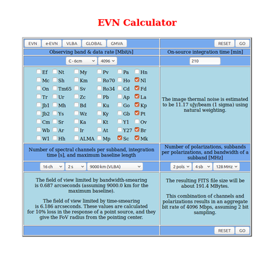 |
|---|
| Example of using the EVN Exposure Calculator. Notice that only 8 antennas are selected. This is because the (hypothetical) proposal states that a minimum of 8 antennas are required for the project to be successful. |
Time on Source: Note for 3mm Observations
The 3mm noise estimates provided by both the EVN Observation Planner and the old EVN Calculator use System Equivalent Flux Density (SEFD) values determined during reasonably good weather and while the antennas were performing well. Because real-world conditions are often less than ideal, the actual noise levels obtained during 3mm observations may be significantly worse. This is especially true for GMVA observations, which are observed on fixed dates and cannot be rescheduled due to poor weather. When planning for GMVA observations, users are encouraged to assume the actual noise values will be roughly 3 times higher than the tool's estimate.
Time on Source: Subbands vs Basebands
There is a subtle difference between how the sensitivity calculator tools and the NRAO PST Resources determine data rates. Both the EVN Observation Planner and the old EVN Calculator ask you to input the number of polarizations and subbands, while the PST Resources ask for the number of polarizations and data channels (formerly called "baseband channels"). Keep in mind that the number of data channels = (number of observed polarizations) x (number of subbands). In other words, for dual polarization, each subband has one left-hand circularly polarized (LCP) data channel and one right-hand circularly polarized (RCP) data channel. For full polarization (“4 pols”), only 2 polarizations are recorded during the observation and the cross-hand polarizations are determined during correlation, so the recorded data rates for “2 pols” and “4 pols” are identical.
To use either the EVN Observation Planner or the EVN Calculator to simulate a 4 Gbps DDC dual-polarization observation: select 4 subbands, 256 (or more) spectral channels per subband, and 2 polarizations.
To simulate a dual-polarization PFB observation: select 16 subbands, 64 (or more) spectral channels per subband, and 2 polarizations.
Time on Source: Spectral Line Observations
The EVN Calculator was designed primarily for continuum observations. If your project involves spectral line observations, you will need to make some additional calculations to estimate the noise in each spectral channel. The per-spectral-channel noise is the noise for the full bandwidth multiplied by the square root of the total number of spectral channels.
For example, assume you observe with 8 data channels per polarization and a data channel bandwidth of 32 MHz. If you want 125 kHz spectral channels, you will need to have 2048 spectral channels in each data channel (8 x 32 MHz / 125 kHz = 256 MHz/125 kHz = 2048). So, the per-spectral-channel noise would be the noise for the full bandwidth times the square root of 2048.
The new EVN Observation Planner provides the per-spectral-channel sensitivity along with the continuum sensitivity.
Time on Source: U-V Coverage
For some projects, particularly those attempting to image complicated structures, filling in as much of the u-v plane as possible may be a greater concern than the sensitivity. If this is the case for your project, be sure to make a note of this in the Technical Justification. Note that the EVN Observation Planner provides an estimate of the u-v coverage for an observation on the UV Coverage tab.
Full Bandwidth vs. Usable Bandwidth
Continuum observations at lower frequencies (at wavelengths of about 13 cm and longer) often encounter problems with RFI. In some cases, large portions of the bandwidth are completely dominated by RFI and are unusable for science. If you are proposing for a low frequency project, it is prudent to assume that the usable bandwidth will be substantially reduced (by up to about 30%). Therefore, the time on source necessary to achieve your desired image thermal noise will be significantly longer than the EVN Observation Planner predicts. If you are asking for more time than the EVN Observation Planner predicts is necessary, make sure to explain why in the Technical Justification.
For example, "The EVN Observation Planner predicts a time on source of 120 minutes will result in an image thermal noise of 25 microJy/beam. However, this is assuming the entire 256 MHz, dual polarization bandwidth at 21 cm will be usable. We anticipate that approximately 30% of the bandwidth will be unusable due to RFI, and therefore we will require 172 minutes on source to reach the necessary signal-to-noise ratio."
Overhead and Total Time
When proposing for time on the VLBA (and other NRAO telescopes), you must request the total time needed for the entire project. This is not just the time on science targets. It also includes time for observing calibrators, time slewing between sources, and the time it takes to change from one frequency setup to another (if you are observing with multiple bands in a single observation).
Estimating Total Observing Time
A “rule of thumb” is that, for a phase referencing observation, the time spent on the science target will be roughly 60% to 70% of the total observing time. The other 30% to 40% of the time will be spent slewing and observing calibration sources. So, to make a conservative estimate of the total observing time you would divide the desired on-source time by 0.6. However, users should be extremely cautious about blindly using this estimate. It only works for projects at low frequencies observing a single science target and phase reference calibrator. Most observers also schedule time on a "check source", a known bright source that can be used to test how well the calibration worked. If your project involves multiple science targets, the project will have more slew time. If your project requires polarimetry, you will also need to schedule scans on polarization leakage (D-term) and electric vector polarization angle (EVPA) calibrator targets. If your phase reference calibrator is relatively far from your science target, the slew time will be longer. If you are observing at high frequencies, you will need to cycle back and forth between the phase reference calibrator and the science target at a higher cadence which adds more slew time. In other words, the more complicated a project, the more overhead it will require.
The best way to estimate the total observing time is to build a dummy schedule with SCHED (see Chapter 6). If you do not know the location of your science target (e.g., for a triggered target of opportunity project), make some reasonable assumptions about where it could be (e.g., classical novae are most likely to be located near the Galactic Center). Then, make some assumptions that would add complications to the schedule. For example, assume that the science target does not have a phase reference calibrator very near by so the slew times will be longer.
To get started, you may use this example dummy.key scheduling file for a hypothetical phase referenced project. In the "In line source catalog", change the DUMMYTARGET source to your science target (and add others as needed). In "The Scans" section at the end, check that that all of your sources are included in the first group and make sure to change the group number if you have more than one science target. Change the phase reference source and check source to something realistic for your project. You will probably need to change the start time and/or date in the "Initial Scan Information" section, as well.
Note that the dummy.key file is built for a “typical” 5 GHz phase referenced observation with 3-minute scans on the science target and 2-minute scans on the phase reference calibrator. This assumes that the phase reference calibrator is relatively dim and requires 2 minute scans to achieve the necessary signal-to-noise ratio of 7. Many observers use significantly shorter scans on the phase reference calibrator, with scans as short as 30 seconds reasonable for brighter calibrator sources.
The cycle time (a.k.a. “switching time”) for a phase referenced observation is the time between the midpoints of two successive scans on the phase reference calibrator with one scan on the science target in between (i.e., cal, sci, cal). The cycle time should be no longer than the coherence time, which depends on your observing frequency. The dummy.key file assumes a coherence time of about 5 minutes: (120 seconds on phase calibrator)/2 + 180 seconds on science target + (120 seconds on phase calibrator)/2 = 300 seconds = 5 minutes. For frequencies below 1 GHz, assume a coherence time of about 2 minutes. At frequencies between 1 and 3 GHz, assume the coherence time is about 5 minutes. For frequencies at or above 5 GHz, you can estimate the coherence time using t[seconds] ~ 2300/frequency[GHz] (e.g., Reid & Honma 2014). Also, keep in mind that the coherence time depends on the elevation of the source, with observations at lower elevations having shorter coherence times (e.g., Ulvestad 1999). For the best results, observers are strongly encouraged to use the cycle times given in Table 1 of Wrobel et al. (2000):
1 GHz to 8.4 GHz: 300 seconds
15 GHz: 120 seconds
22 GHz: 60 seconds
43 GHz: 30 seconds
Once you have made all the changes to the dummy schedule, run SCHED on it by typing
sched < dummy.key
and inspect the summary (dummy.sum) file to see the total time for the observation (“Elapsed time for project”) and the total time on your science target(s). Change the number of repetitions (rep=#) and/or dwell times under "The Scans" and re-run SCHED until you settle on a schedule that gives you the desired time on your science target(s).
If you have any questions about determining the on-source time, building a dummy schedule, or running SCHED, please contact the VLBA staff via the helpdesk.
Technical Justification
Many new (and even some experienced) VLBA users are intimidated by the Technical Justification (TJ) portion of the Proposal Submission Tool (PST). However, it may be better to view the TJ section as an opportunity to move some of the technical details out of the Science Justification and make room for more science.
The TJ consists of several sections where users are required to enter brief statements about the technical nature of their proposal. Essentially, this is where users demonstrate that their proposed project is technically feasible and that they have considered various difficulties that may arise.
As you write your science justification, or as you read one that someone else wrote, keep in mind that some details about the planned observations can be put in the TJ instead. It may even be useful to fill in (or at least start to fill in) the TJ before you begin writing the science justification in order to avoid repeating yourself.
The Science Review Panel (SRP) and the Time Allocation Committee (TAC) will both have access to the TJ associated with a proposal. An NRAO staff member will review your TJ before your proposal is given to the SRP. The SRP and the TAC will both have access to any comments from the NRAO Technical Reviewer.
Technical Justification Sections
Stations Requested: Proposers should specify the minimum number of stations needed to achieve their science goals. Also, list any individual stations that are required. Proposers often state that they require both MK and SC in order to get the best possible angular resolution. If Y1 or any HSA stations are needed, explain why they are necessary. It is generally a good idea to assume that at least one, and probably two VLBA stations will be unavailable at any given time. Additionally, triggered proposals that require a rapid response (~1 week or less) should consider only requiring seven stations, only one of which should be an island site. If a proposal states that it requires all ten VLBA stations, it may be difficult to schedule because at least one station is often unavailable due to mechanical problems, poor weather, and/or network issues.
Future Semesters: If the proposed project will require observations in 2 or more semesters, explain why here.
Receivers: List all receivers that will be used, and provide a brief justification for those choices.
Scheduling Issues: List any restrictions on when or how the observations can be done. This includes specifying exact dates for fixed-date projects, stating the minimum length of scheduling blocks, and specifying what weather conditions are acceptable.
Correlator Setup: This section is used to specify what the correlator will do with the data after it has been taken. This should include integration times, observation type (continuum, spectral line, or pulsar), and any other details about the correlation. For example, if the project requires more than one phase center, state that here. NOTE: The recording data rate is not related to the correlator, so you do not need to say anything about "4 Gbps" or "2 Gbps" here.
Self-calibration: State whether or not the science targets are expected to be bright enough for self-calibration. If not, specify which phase reference calibrators you plan to use (if known). If you will need extra time on either the VLA or VLBA to identify good phase reference calibrator sources for your project, you can request that time here.
Sensitivity Required: Clearly state what sensitivity is needed to achieve the science goals. For example, "An image rms of 40 microJy/beam is necessary to detect the core at the 5-sigma level, but we expect the jet component to be much dimmer. We therefore require a sensitivity of 5 microJy/beam."
Integration Time: In this section, state the on-source integration time needed to achieve the sensitivity stated in the previous section. You will also need to provide a screen shot of the EVN Calculator or the pdf from the EVN Observation Planner. If your project will involve observations with more than one receiver, you will need to include a calculator estimate document for each band. NOTE: When calculating the exposure time, remember to use the minimum number of antennas you specified in the first section of the TJ.
Sensitivity or Dynamic Range Limited: Clearly state whether you expect your results to depend on the sensitivity or the dynamic range. If this section is left blank or has "NA", the Technical Reviewer may write something like "This project appears to be sensitivity limited". If you do not want the Reviewers making guesses about your project, make sure you enter something here.
Polarization: If you plan to do any polarimetry with your observation, you may require some VLA observations of polarization calibrators near the time of you VLBA observation. List any calibration sources you intend to use here.
Flux Calibration Accuracy: If you need flux calibration accuracy better than about 10%, state that here and explain how you will achieve this accuracy.
Total Correlator Output Data Size: Give you estimate for the total size of all FITS files that will result from your observation. This should account for all targets (both calibration and science) and all epochs.
Joint Proposal Details: For joint proposals, you will need to enter some extra technical information about the other instrument(s) you requested.
Min/Max GST: If you do not use the default GST range from the Sources section, you will need to explain why here.
Other Considerations: If your project has any additional needs, list them here.
Common Mistakes
The most common mistake proposers make in the TJ section is to miscalculate the time on source necessary for their project. Many times, the proposer will use the EVN Calculator or EVN Observation Planner with all 10 VLBA antennas, but then state that their project can be done with only 8 (or fewer) antennas. This is not always a problem, but it can lead to Technical Review comments like:
“The proposers state that only 8 antennas are needed for the observations, but the on-source time estimate was made using 10 antennas in the EVN Calculator. It is unclear that the requested time is adequate to successfully complete the project with the minimum required number of antennas.”
Another common mistake is when users who are proposing for L (21 cm, 1 GHz) or S (13 cm, 2 GHz) band observations do not take into account the impacts of RFI in those bands. RFI is increasingly a problem at those frequencies and it will have an impact on the usable bandwidth, which results in a reduction in sensitivity. Proposers should assume that between 20% and 30% of the bandwidth will be unusable at L and S bands, an adjust their sensitivity estimate accordingly (see the Exposure and Overhead chapter).
One more common mistake is when a proposer states that they need flux density calibration accurate to 5%, but they do not provide any information about how they will achieve this accuracy. The nominal VLBA flux density accuracy, with standard calibration techniques, is about 10%.
Comments from a Technical Review can impact the SRP’s ranking of projects. Proposals that do not appear technically feasible are often given lower rankings. However, these comments are not always detrimental to a proposal. If the science justification is compelling and the SRP rates the proposal highly, a comment about the on-source time estimate on the TJ could lead to the TAC granting more time than what was requested in order to ensure the project’s success. The Technical Review is not intended to determine which proposals are granted time, but to ensure that successful proposals lead to successful observations.
If you have any questions about the Technical Justification section, please contact NRAO staff via the helpdesk.
Example
Below is an example of a filled TJ is presented below. The example project involves VLBA antennas only (no HSA, no Global VLBI).
 |
 |
| Example of a completed Technical Justification section of the PST. Click on the images for the full-size versions. |
Submission Guidelines
The following guidelines are designed to assist in the submission of proposals into the Proposal Submission Tool (PST). There are two sets of guidelines, one for General and Shared Risk Observing (GO / SRO) and one for Resident Shared Risk Observing (RSRO); note that while some of the steps to completion are the same between GO / SRO and RSRO, the latter has additional considerations that need to be taken into account before submission of the proposal.
General and Shared Risk Observing (GO / SRO) Steps to Completion
- Read the current Call for Proposals description for summaries of the capabilities being offered for GO and SRO.
- Review the NRAO User Portal and Proposal Submission Guide for details on the online tool and proposal submission policies (proposal types, page limits, etc...).
- Write a scientific justification for your proposal. Note that technical information should be included in the Technical Justification section form and does not need to be included with the scientific justification. Save your scientific justification as a PDF file.
- Use the EVN Exposure Calculator to determine the required sensitivities. Remember to use the appropriate number of antennas. In general, it is best not assume you will get all 10 VLBA antennas, unless this is required by your proposal.
- Determine the total time to be requested, including all overheads.
- Log into the NRAO Interactive Services page and click on the Proposals tab in the top left to create a new proposal for the VLBA. Once you are in the tool, extensive help is available in the tool by clicking on the Help button in the top right of the tool interface. In the Proposal Submission Tool (PST):
- Fill in the relevant fields for each section of your proposal;
- If you are proposing for continuum observations, select Observing Type = Continuum in the General section of your proposal. Then add a Continuum Resource, selecting the appropriate band you want to observe in. Default optimum continuum setups for each band are defined in the PST.
- If you are proposing for spectral line observations, select Observing Type = Spectroscopy in the General section of your proposal.
- Upload your scientific justification as a PDF file;
- Click on the Technical Justification page in the proposal and fill in the appropriate boxes (example of technical justification). In order to determine sensitivities, you will need to use the EVN Exposure Calculator Tool to understand what sensitivity you will get for a given observing band, bandwidth, antenna set, and integration time. If you have trouble running the EVN Exposure Calculator please contact the NRAO Helpdesk. If you have a reason for not used the EVN Exposure Calculator, state it in the box asking for the screenshot.
- Note that the PST allows observers to specify multiple resource types (e.g., you can have one proposal that specifies general and/or RSRO correlator resources). If any resource is RSRO then the proposal will become a RSRO proposal.
- Fill in the relevant fields for each section of your proposal;
- When your proposal is complete, validate it to make sure there are no obvious omissions or mistakes. Also double check that the numbers used in the Scientific and Technical Justifications match those provided in any attachments (e.g., EVN Calculator screen shot).
- When you are satisfied, submit your proposal in the PST. Note that proposals can be withdrawn and resubmitted before the deadline.
Resident Shared Risk Observing (RSRO) Steps to Completion
- Read the current Call for Proposals for a summary of the capabilities being offered for GO and SRO. If you want more than what is offered for GO or SRO then you are requesting a RSRO capability (one that is not well-tested and may need additional development). If you propose for a RSRO capability, you—or an experienced person on your team—must be able to participate in the RSRO program by coming to Socorro to help with the development and testing process.
- Review the NRAO User Portal and Proposal Submission Guide for details on the online tool and proposal submission policies (proposal types, page limits, etc...).
- Write a scientific justification for your proposal. Note that technical information should be included in the Technical Justification section and does not need to be included with the scientific justification. Save your scientific justification as a PDF file.
- Log into the NRAO Interactive Services page and click on the Proposals tab in the top left to create a new proposal for the VLBA. Once you are in the tool, extensive help is available in the tool by clicking on the Help button in the top right of the tool interface. In the Proposal Submission Tool (PST):
- Fill in the relevant fields for each section of your proposal;
- Even as a RSRO proposal, you will need to create a Resource in the PST and select the VLBA RSRO Observing Mode. This will give you a text field in which you can type a description of your setup;
- Upload your scientific justification as a PDF file;
- Technical justifications are now included as a separate section in the proposal. Click on the Technical Justification page in the proposal and fill in the appropriate boxes (example of technical justification). Describe what you want to do with the correlator and why this is in the RSRO Category in this section. Contact NRAO staff if you have questions about exactly what is feasible. The last box at the bottom of the Technical Justification page should be used to describe your RSRO effort. Identify who in your team will help commission this capability and how their background and expertise can be applied to this development. Working with NRAO staff, estimate the level of effort that is likely to be needed for this development and specify how long a member of your team can devote their time for this effort (either by visiting NRAO-Socorro, or doing the work remotely).
- Note that the PST allows observers to specify multiple resource types (e.g., you can have one proposal that specifies general, shared-risk and RSRO correlator resources). If any resource is RSRO then the proposal will become a RSRO proposal.
- When your proposal is complete, validate it to make sure there are no obvious omissions or mistakes.
- When you are satisfied, submit your proposal in the PST. Note that proposals can be withdrawn and resubmitted before the deadline.
RSRO Considerations
A RSRO proposal should contain:
- A scientific justification, to be peer reviewed as part of NRAO's current time allocation process, submitted through the Proposal Submission Tool. Note that RSRO correlator resources should be specified as plain text on the Resources page in the PST by selecting WIDAR RSRO as the backend.
- A technical justification, to be be reviewed by NRAO staff, which should include:
- A list of the personnel who will be involved in the effort and a description of how their expertise will be used to address the critical priorities of VLA development relating to their proposal.
- The proposed dates of the residency or remote participation, so that these can be matched to VLA development planning.
- A statement of the benefit of the proposed capability to the community.
- A clear description of the scope of the proposed RSRO work, and what will be needed to eventually bring the new capability into SRO status. This will be used to estimate the NRAO resources needed.
Limited support for accommodation in the NRAO Guest House for participants in the RSRO program may be available.
The acceptance of a RSRO proposal will depend on the outcome of the time allocation process. Proposals will also be evaluated by NRAO staff in terms of the priorities and benefits to the VLBA development and commissioning activities.
The primary requirement of the RSRO program is that at least one expert from each participating group will devote their time and contribute to commissioning, while incurring as little overhead from VLBA staff as possible. Limited support for accommodation in the NRAO Guest House for participants in the RSRO program may be available.
In general, one month of dedicated commissioning effort is expected for every 20 hours of VLBA time awarded to a RSRO project, subject to negotiation. While there is no minimum requirement, ideally the dedicated effort should be for about 2 months. However, the amount of time spent to help develop the program should be realistically matched to the expected effort, including time to become familiar with relevant technical aspects. The duration of the dedicated effort should be discussed with NRAO staff to determine what is reasonable. The length of time a RSRO expert should be needed by NRAO may be on the order of a few months.
The period(s) of participation (in person) may occur in advance of the observing time awarded in order to decouple essential scientific requirements from other factors which may affect when personnel are available (such as teaching schedules). However, observers should be available for one week prior to their observations in order to become familiar with the latest developments and to set up their observations. In the special case of Target of Opportunity proposals, a VLBA staff collaborator may be required for setting up observations on short timescales.
It is also possible for a member of the NRAO scientific staff to satisfy the residency requirement on a RSRO proposal. NRAO staff considering providing the residency requirement for an RSRO proposal should consult with their supervisor for further information. Graduate students may lead a RSRO project, provided relevant expertise is demonstrated in the RSRO relevant sections of the proposal. Graduate students should be accompanied by their advisor at the start of their in-person or remote participation. RSRO participants will work under NRAO management in order to optimize the overall commissioning effort. A set of deliverables will be agreed upon in advance of the start of the residency.
The types of proposals considered under the RSRO program may include both large (>200 hours) and small (~10–200 hours) projects. Qualified large projects proposed by consortia will be considered as long as the RSRO requirements are met. A single individual may satisfy the RSRO requirement for several small projects.
RSRO participation without a science proposal
In some cases an individual may want to participate in development activities without writing a science proposal. A participant may arrange to visit Socorro to contribute to development activities by submitting a proposal of who will come and the technical development to be undertaken directly to the Assistant Director for New Mexico Operations (nraonmad@nrao.edu). If the Assistant Director approves of the request, then the individual may come to Socorro to contribute to development activities. The participant may then obtain observing time either by submitting a proposal at a regular proposal deadline, or by submitting an Exploratory Proposal through Director's Discretionary Time. Such visits should conform to the residency requirements above. Proposals to visit Socorro under this program may be submitted at any time.
Frequently Asked Questions
Bandwidth and Noise
What bandwidth should I use for noise calculations?
If you are doing a spectral-line project, you need to determine the noise per channel. To do this, take the noise over the entire bandwidth (as reported by the EVN Sensitivity Calculator), then multiply by the square root of the number of channels. (For an example, see Slide 46 in the 2019 VLA and VLBA Proposal Preparation presentation by Emmanuel Momjian.)
If you are are doing a continuum detection experiment, in which you want to cover as much spectral range as possible, use the total (RFI-free) bandwidth. When in doubt, use the total bandwidth you plan to use in making an image. For high frequencies this is usually the entire bandwidth.
Polarization Products and Noise
How does the number of polarization products affect the noise?
Choices are single polarization (RR or LL), dual polarization (RR and LL), and full polarization (RR, RL, LR, and LL). If the emission is unpolarized, dual polarization gives twice the amount of independent data as single polarization does, and therefore decreases the rms noise by a factor √2, as the sensitivity calculator will show. Full polarization does not improve this any further since RL and LR do not contribute to Stokes I. For most cases you will want dual or full polarization.
Phase Referencing
When should I use phase referencing?
If there is any chance that your science target will not be bright enough for self calibration, you should use phase referencing. You should also use phase referencing if you are interested in the absolute position of the target, even if it is bright enough for self calibration.
Calibrators
How should I pick calibrators for my project?
The new VLBA Calibrator Search Tool will provide you with a list of potential calibration sources. It is generally a good idea to check for recent information on these sources to ensure that variability is not an issue at your desired observing frequency. An ideal calibrator source has significant flux density on all the baselines that will be used for a project. Also, check that the positions of the sources are known to an acceptable uncertainty for your project. If you cannot find recent information on calibrators at your desired frequency, you can request extra observing time to identify a good calibrator (see the Technical Justification section regarding whether targets can be self-calibrated).
An alternative search tool is the NASA VLBI Calibrator Search tool, which is particularly useful for those interested in the history of a source's flux density measurements.
What calibration sources do I need for polarimetric observations?
Polarimetric observations require three types of calibration:
- Leakage (D-term) calibration: To calibrate the D-terms you will need scans on a strong (~1 Jy) calibrator, preferably one with little structure. Popular D-term calibrators are OQ208 (J1407+2827) and DA193 (J0555+3948). If an unpolarized source is chosen for the D-term calibrator, only a single scan is necessary. If the D-term calibrator has any polarized flux, at least 5 calibration scans should be made covering as large a range in parallactic angle as possible. You can plot the parallactic angle coverage in SCHED.
- RCP-LCP delay calibration: Observe at least one 2-minute scan on a very bright (~10 Jy) polarized calibrator. The goal here is to be able to detect fringes on the cross-hand (RL and LR) correlations so a significant amount of polarized flux is required.
- Electric vector polarization angle (EVPA) calibration: Observe at one electric vector polarization angle (EVPA) calibrator (although 2 or 3 EVPA calibrators are recommended).
It is possible that some of these calibrators can be the same source, like using one source for both RCP-LCP delay and EVPA calibration. For obvious reasons you cannot use an unpolarized calibrator to calibrate the D-terms and use that for the other two calibrations. See the VLBA Polarimetry page for more details.
Overhead
What overhead should I count on for slewing, calibration, etc?
The best way to estimate the total time needed for an observation is to build a dummy schedule in SCHED. Make sure to include scans on any calibration sources.
Setup Restrictions
How do current observing setup restrictions impact my proposal?
There are a number of observing constraints with the 2 VLBA observing modes. Most of these become important when preparing the observing script, but the following are of potential interest to proposers as well.
- The VLBA receivers can only be set to certain allowed frequencies. Check the SCHED example setup files for examples of how to tune the frequencies in your obseravtion.
- If a target is observed at multiple frequencies during a single observation, there will be increased calibration overhead since it takes a finite amount of time for the telescope to switch receivers. For phase reference observations, each target source scan at a certain frequency has to be bracketed by gain calibrator scans at that frequency.
Assistance with VLBA Observations
Can I get help setting up observations, calibrating and analyzing my VLBA observations?
Users can always use the NRAO helpdesk for assistance with any issues related to any of the telescopes operated by NRAO. VLBA staff are available to provide assistance with proposal preparation, schedule creation, and data reduction.
VLBA users are also encouraged to visit the NRAO in Socorro, NM, for face-to-face assistance with calibrating and reducing their observations. Travel support is available. Please note that current NRAO policy requires all visitors to provide proof of vaccination against the COVID-19 virus.
There are also on-line data reduction tutorials.
Past Approved Proposals
A Proposal Finder Tool (PFT) may be used to search cover sheets of proposals previously approved for time on NRAO telescopes. See also active triggered proposals, large proposals, and approved Director's Discretionary Time (DDT) proposals.
Acronyms
AUI = Associated Universities, Inc. (the managing body of NRAO)
DDC = Digital Downconverter
DDT = Director’s Discretionary Time
EVN = European VLBI Network
EVPA = Electric Vector Polarization Angle
GBT = Green Bank Telescope (officially, the Robert C. Byrd Green Bank Telescope)
GMVA = Global Millimeter VLBI Array
GO = General Observing
GST = Greenwich Sidereal Time
HSA = High Sensitivity Array
IEEE = Institute of Electrical and Electronics Engineers
LCP = Left-hand Circularly Polarized
LST = Local Sidereal Time
NRAO = National Radio Astronomy Observatory
NSF = National Science Foundation
OSS = Observational Status Summary (Note: the VLBA and VLA each maintain their own separate OSS.)
PFB = Polyphase Filter Bank
PFT = Proposal Finder Tool
PST = Proposal Submission Tool
RCP = Right-hand Circularly Polarized
RDBE = ROACH Digital Backend
RFI = Radio Frequency Interference
ROACH = Reconfigurable Open Architecture Computing Hardware
RSRO = Resident Shared Risk Observing
SEFD = System Equivalent Flux Density
SRO = Shared Risk Observing
SRP = Science Review Panel
TAC = Time Allocation Committee
TEC = Total Electron Content
TJ = Technical Justification
ToO = Target of Opportunity
UHF = Ultra High Frequency
VHF = Very High Frequency
VLA = Very Large Array (officially, the Karl G. Jansky Very Large Array)
VLBA = Very Long Baseline Array
VLBI = Very Long Baseline Interferometry
NRAO Bands: Letter Codes and Frequencies
One of the most confusing aspects of radio astronomy for new students is the naming convention for the different radio bands. The letter designations for the bands do not appear to make any logical sense. Why is P-band a lower frequency than L-band, but S-band is a higher frequency than L-band? The story most of us are told is that the band letter designations were created during World War II. The Allies were using radar for aircraft detection and tracking, and (of course) radio for communications. To confuse the Axis powers, the Allies gave secret letter designations to the various frequency bands they were using. To further confuse the Axis, those letter designations were not assigned in alphabetical order, and lower-case sub-band designations were often added. This meant that a radio operator who suspected their transmission was being intercepted could tell other operators “switch to Ku”, and the Axis would not necessarily know which frequency to change to in order to intercept the rest of the communication. For radar, it meant that even if the Axis discovered that a particular radar operated at X band, they did not know the specific frequency they would need to broadcast in order to jam it.
There may have been some logic to the letter designation. For example, “S” may have stood for “short wave” and “L” may have stood for “long wave”. “P” is said to have meant “previous”, because the British originally operated radars in the 250–500 MHz range before switching to higher frequencies. “C” is said to have stood for “compromise” (between S and X). Radars that operated at X band were often used for fire control, so “X” is said to be a reference to a crosshair.
Unfortunately, these historical explanations do not seem to be documented anywhere. According to some sources, the US government never declassified the documents relating to the frequency designations.
What is documented is the fact that the International Telecommunications Union adopted official band designations in 1959. However, these designations only covered frequencies up to 40 GHz.
In 1984, the IEEE adopted official radar frequency letter designations for frequencies from 3 MHz to 300 GHz. These designations were updated in 2019.
The table below shows the NRAO frequency band designations, which mostly (but not quite always) follow the IEEE standard. The NRAO P and Q bands are not official IEEE bands; P spans the upper end of the VHF band and lower end of the UHF band, and Q covers a portion of the IEEE V band. The “Associated Wavelength” for each band often depends on who you are talking to, the specific telescope they are talking about, and what their scientific interests are.
|
Band Designation |
Frequency Range |
Associated Wavelength(s) |
|---|---|---|
| 4-band (VLA only) | 58 – 84 MHz | 4 m |
| P | 220 – 500 MHz | 90 cm |
| UHF (VLBA only) | 596 – 626 MHz | 50 cm |
| L | 1 – 2 GHz | 18, 20, or 21 cm |
| S | 2 – 4 GHz | 13 cm |
| C | 4 – 8 GHz | 6 cm |
| X | 8 – 12 GHz | 3, 3.6, or 4 cm |
| Ku | 12 – 18 GHz | 2 cm |
| K | 18 – 26.5 GHz | 1.3 cm |
| Ka (VLA only) | 26.5 – 40 GHz | 1 cm |
| Q | 40 – 50 GHz | 7 mm |
| W (VLBA only) | 80 - 90 GHz | 3 mm |
NOTE: The VLBA receivers often do not cover the entire frequency range of a given band. See the Frequency Bands & Performance section of the OSS for details on the VLBA receivers.


Connect with NRAO