OPT Manual Complete Manual
Overview of the Observation Preparation Tool Manual
Introduction and Purpose of the Manual
This manual describes the web application used for creating observing schedules for the Karl G. Jansky Very Large Array (VLA). It is not intended to teach observing strategies and good observing practices. For that information, please refer to the Observational Status Summary (OSS), Guide to Observing with the VLA, and other VLA documentation. If you have any questions, please submit them to the NRAO Science Helpdesk.
An observing schedule is created using the Observation Preparation Tool (OPT) Suite*, a web application consisting of three separate tools that are used in conjunction. The reader will be guided through the three tools and provided detailed information on how to create an observing schedule and how to submit it.
- Source Catalog Tool (SCT): define and select positions on the sky.
- Resource Catalog Tool (RCT): define and select hardware (receiver and correlator) settings.
- Observation Preparation Tool (OPT): define and create a sequence of scans. A scan is a combination of an observing mode, a source, a resource, a time interval, and scan intent(s).
*The Observation Preparation Tool (OPT) Suite is a product of the National Radio Astronomy Observatory staff. The Karl G. Jansky Very Large Array (VLA) is operated by the National Radio Astronomy Observatory (NRAO), which is a facility of the National Science Foundation (NSF) operated under cooperative agreement by Associated Universities, Inc. (AUI).
Abbreviations Used
When referring to the OPT in the remainder of this document, it is implicitly referring to the tool that creates a sequence of observing scans. On the other hand, when we refer to the OPT Suite, we specifically refer to the combination of tools consisting of the SCT, RCT, and OPT.
The use of the term '(re)source' is short-hand for the text "source and resource": the sentence applies to both source and resource. Similarly, using 'project (etc.)' allows us to avoid having to write "project, program block(s), scheduling block(s), and scan(s)" which otherwise would make sentences confusing. For program block and scheduling block we will use PB and SB, respectively, or blocks when we mean either or both.
We will also use PST (Proposal Submission Tool) and TAC (Time Allocation Committee), which have some interaction or influence on what goes on in the OPT Suite.
The OPT Suite
Introducing the Tools
To access the OPT Suite, go to the NRAO User Portal. You will be required to login or create an account. If you have forgotten your password, you may reset it, if you have forgotten both username and password, please create a new account to contact us via the NRAO Science Helpdesk. Do not use the registration owned by someone else.
After logging in to the NRAO User Portal, click on the Obs Prep tab at the top. This will redirect you to a dashboard containing a link to Login to the Observation Preparation Tool (OPT). Note you may also access the OPT Suite directly by using this url: https://obs.vla.nrao.edu/opt. In the web application you will see a menu bar (above the white line) and a navigation bar (below the white line) (see Figure 1.2.1). The web application opens to the OPT (labeled as Observation Preparation). You can also navigate to the SCT and RCT in the navigation bar using the links labeled Sources and Instrument Configurations, respectively. We have tried to keep the editing concepts as similar as possible across the three tools.
 |
|---|
|
Figure 1.2.1: OPT Suite menu and navigation bar. |
The OPT Suite is a web application written in JAVA. This allows us to keep an up-to-date production version for all users. However, this can also cause slowness since it is actively connecting and interacting with the NRAO database. For the best performance, we recommend using Firefox as the web browser. The OS of your computer should not matter. After a certain amount of inactivity the web application will time out; however it will auto-save any changes made. To exit gracefully go to File and choose Exit, or find the Exit button at the top right. Please do not exit the tool by closing the web browser or browser tab before exiting properly, with either of the exit options, as this will keep your session active and will create problems accessing your project for some hours.
The most important rule when working in the OPT Suite: be patient. When you click on something or enter information into a field it may take a few seconds to connect back and forth between your browser and the NRAO database. Please avoid clicking or entering before the previous action was completed. Be patient and watch the busy icon of your browser to stop (and sometimes even a bit longer). If you continue to have problems, contact us through the NRAO Science Helpdesk.
The SCT, RCT, & OPT
The SCT (https://obs.vla.nrao.edu/sct), labeled as Sources in the navigation bar, is used to specify a collection of telescope pointing directions, i.e., a source position on the sky from which the user can select when creating a list of scans in the OPT.
The RCT (https://obs.vla.nrao.edu/rct), labeled as Instrument Configurations in the navigation bar, is used to specify a collection of hardware and instrument configurations from which the user can select when creating a list of scans in the OPT.
The OPT (https://obs.vla.nrao.edu/opt), labeled as Observation Preparation in the navigation bar, is used to setup an observation, i.e., a Scheduling Block (SB), by creating a list of scans containing sources, resources, and scan intents. Each scan consists of a source position (selected from the SCT) using a specific hardware and instrument configuration (selected from the RCT) combined with an observing mode action lasting for a time interval, and for a specific reason (scan intent(s)).
Projects, Program Blocks, & Scheduling Blocks
The OPT contains three levels:
- Project level contains the project code (e.g., 20A-001 or SF1234), the PI, co-I’s, and total allocated time.
- Program Block (PB) level contains hours allocated to a specific array configuration (e.g., A, B, C, D, or Any) in the allocated observing semester and observing priority (e.g., A, B, or C), and Execution Block(s) (EB) once an observation has been run (successfully or unsuccessfully).
- Scheduling Block(s) (SB) are created within the PB and can be linked using the conditional format system (to be described in more detail in the OPT section).
The Project level will consist of at least one PB and within the PB will contain any number of SBs created by the observer. Typically a PB does not extend to another observing semester. For example, if you were allocated time for the A-configuration and B-configuration, then one PB will be defined for the A-configuration and one for B-configuration, perhaps in a following semester. You may also find PBs for the same array configuration but with time allocations split over different observing priorities.
SBs may be many different snippets of an observing run, i.e., groups of consecutive scans that constitute a complete observation totaling the allocated time. Or an observing run may also be defined in a single SB. In both examples, the observed SB(s) would complete the allocated time within a specific PB. These observing methods would depend on what the user finds appropriate for their science and observing priority.
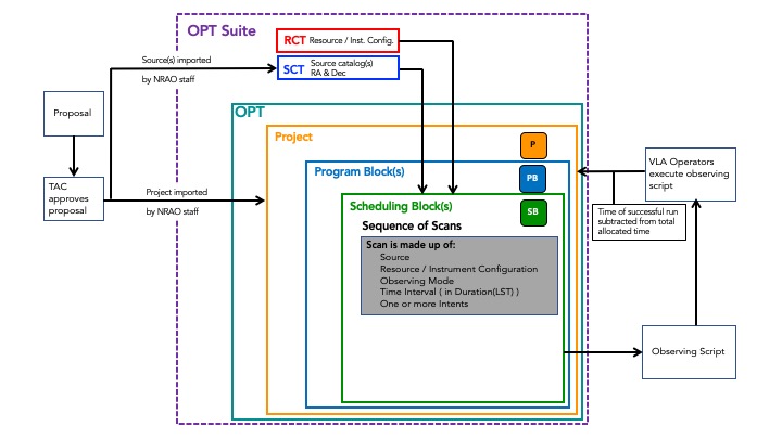
The Flow of an Approved Proposal to Observed SBs Explained (Figure 1.2.2):
After a proposal has been submitted, reviewed, and approved by the Time Allocation Committee (TAC), NRAO staff import the project into the OPT about a month before the start of the allocated configuration. During this process, the source list provided in the Proposal Submission Tool (PST) will be imported into the SCT. In the future, this will happen for resources supplied in the PST as well, but for now they have to be created in the RCT by the user.
In the RCT you may use the NRAO default resource(s) or create your own resource(s) that you proposed to set up. Inside the project you will find the Program Block(s) (PB) allocated by configuration (A, B, C, D, or Any) and inside the PB, you will find a starter scheduling block (SB) that you may use to create your SB(s).
An SB is a series of scans. A scan is comprised of: a source imported from your personal source catalog or from the VLA Calibration Catalog; a resource / instrument configuration imported from your personal resource catalog or from the NRAO default resource catalog; an observing mode; a time interval in Duration(LST); and one or more observing intents. Once you have created the SB and it passes the first stage of validation to where you can submit it, the data analysts (DAs) will perform a secondary validation of the SB for items such as correct wrap, missing scans, incorrect intents for the scan, etc. When an SB has passed this second and more intensive validation, it will be approved for observation.
When an SB is approved, it is converted from human-readable scans to a machine-readable file (the observing script). This script is then executed by the VLA Operator based upon certain criteria such as the weather constraints (wind and atmospheric phase limit (APL)), observing priority, and other factors. When the observation is successful, the duration of the SB is subtracted from the total allocated time. If for some reason the observation is aborted or failed due to issues with the correlator, array, or weather, the time is not counted against the total allocated time. There are some circumstances where we will not fail an observation if the problem lies in how the SB was setup outside of our recommended guidelines.
 |
|---|
|
Figure 1.2.2: Schematic flow diagram of approved proposal to observed SBs. |
Tool Layout
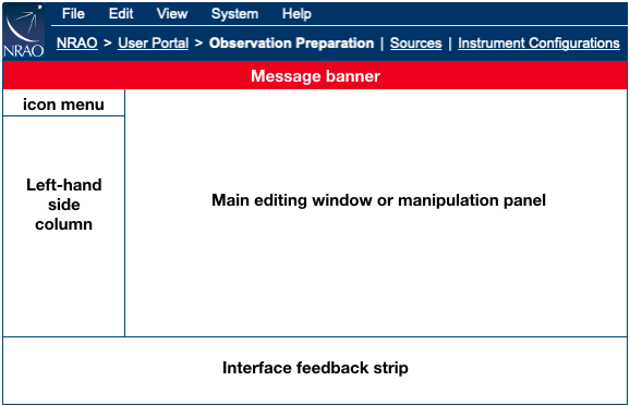
After logging in to the OPT Suite via the NRAO User Portal, you will be presented with the OPT from where you can navigate to the SCT and RCT (see Figure 1.2.1). Each of the tools will display a menu bar and a similar navigation bar at the top. If the tool name is bold with no underline, then that is the current tool in use. The underlined tool names can be accessed by clicking on the name, e.g., Sources and Instrument Configurations (as shown in Figure 1.2.3). In addition to the menu and navigation bar, the OPT Suite is organized with an icon menu, a left-hand side column, a main editing window or manipulation panel, and an interface feedback strip at the bottom. Since each tool is utilized for different purposes, they will each display different information in the panels. More information on using the menu bar items will be discussed in later sections.
 |
|---|
|
Figure 1.2.3: Basic layout of the OPT Suite panels. |
The interface feedback strip is the small panel at the bottom of the OPT Suite. This panel is used to display feedback information such as error messages (red font) and warning messages (blue font) generated when entries made through the web interface are validated. It is advised to pay attention to these messages as it may be the only indication that an SB or resource is faulty. An SB with errors cannot be submitted, but an SB with warnings may be submitted if the observer persists. Please note that the interface feedback strip will include a scroll bar and a button (See All Messages for this Scheduling Block) when there are more warnings and errors to display than fit directly on the visible part of the panel. Clicking on the button will allow you to more easily read the error and warning messages.
Occasionally you may encounter a red message banner just below the navigation bar. We use this banner to convey anticipated downtime, emergency software updates, etc., suggesting you to postpone or finish your work promptly. On this banner, you will see a small ‘x’ to the right of the message. If you click on the ‘x’ it will close the banner until you log back into the OPT. For small computer screens, i.e., laptops, this message banner can get in the way of allowing you to import (re)sources into a scan.
The left-hand column (Figures 1.2.4.a-c) will vary depending on which tool is selected.
 |
 |
 |
| Figures 1.2.4.a-c: Left hand columns for the three tools (SCT, RCT, and OPT) | ||
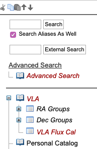
- SCT: At the top of the left hand side column of the SCT, below the icon menu, is an interface to search for sources. The source search is performed on a source name only in the selected source catalog (highlight it by clicking) in the list of catalogs in the bottom part. Alternatively, the source is queried from the SIMBAD database when the external search field and button are used. Check the alias box if you have not entered the name of the source in the selected catalog, e.g., its 3C name. Use Advanced Search if you want to search on something else than a source name in a single catalog, e.g., using a cone search on a position with a flux density limit.
- In the bottom part of the left hand side column of the SCT, there should be at least one source catalog visible in red italics, named VLA that contains the VLA calibrators also in red italics (indicating it is read-only); these catalogs are sorted by RA groups, Dec groups, and VLA Flux Calibrators. There may be other source catalogs visible, e.g., catalogs that you have defined yourself. Small plus-sign icons indicate there are groups of sources defined within a catalog; click on it to expand and display these groups. The VLA catalog also contains subgroups that can be expanded.
- RCT: At least one group of resource catalogs should be visible in the resource catalog column, the NRAO Defaults in red italics (indicating it is read-only). The NRAO Defaults catalog contains the hardware/instrument configurations
- interferometric pointing scans to be utilized for high frequency observing (greater than 15 GHz). (Note, only the NRAO default, X-point (formerly known as X-band pointing), resource should be used for the interferometric pointing scans.)
- 3-bit resources with up to 4 Basebands at 2 GHz bandwidth
- 8-bit resources with up to 2 Basebands at 1 GHz bandwidth
- Alternative resources for A- and B-configuration to reduce the effect of microwave link RFI
- Slew dummies scans for slewing antennas at the start of an SB
- Other resource catalogs may be visible, e.g., a Personal Catalog or any that were previously defined or shared.
- OPT: The left-hand column of the OPT should contain the project for which you were awarded observing time. If the project is not there, please let us know as soon as possible using the NRAO Science Helpdesk. The project is typically entered about a month before the allocated configuration and a readiness email will be sent by the VLA scheduling manager (schedsoc) notifying that the project is available. Other projects may be visible, in particular if you had previous observing programs or if you were awarded observing time for more than one project in this proposal round. Different icons in the tree depict different items: P for projects, PB for program block, SB for scheduling block. When using this for the first time, it may only show the Project; a project tree would be visible all the way to the first scan level with consecutive mouse clicks on the item names in the tree. Some of the information may have been entered from the details of your proposal and should be read-only.
- A small plus-sign icon in front of a project or catalog means that there are items defined within that item; click on it to expand and display a tree-view of these items. For example, clicking on a plus-sign icon in front of a project will expand a list of PBs in that project. Clicking a small minus-sign icon will collapse all content within that item. For speed and memory reasons, not all projects are loaded into memory from the start. If the plus-sign is not visible with the project or SB you would like to work on, simply click the project name to load it into memory.
- At the top of the left-hand side window, there is an icon menu. These icons can be used to cut (delete) or copy and paste specific SBs, individual scans, (re)source catalogs, or (re)source groups. The options of this icon menu act only on the items in the tree, not on the items in the main editing window. In contrast to the small icons in front of a tree item, plus-sign and minus-sign icons in the icon menu expand or collapse the tree under a selected (highlighted) item. Arrow icons move items around in a tree. Navigating between projects, PBs, SBs, and scans in the OPT is simply done by selecting (click to highlight) any such item name in the tree. Similarly, you can navigate between a tool’s catalogs and groups in the left-hand side column trees (in the SCT and RCT).
More on manipulating PBs, SBs, and scans in the OPT, manipulating (re)source catalogs and (re)source groups, and using the source search tool will be discussed in later sections.
The main editing window, or manipulation field, exposes different information fields per tool and per item type. However, the SCT and RCT at first instance will both show a very similar table of catalog contents, i.e., a table of entries in the selected catalog or group.
- SCT: Selecting a source catalog or group within a source catalog will show the sources in this catalog or group in the form of a table listing in the main source manipulation field. If the list contains more than 25 sources, this list will occupy multiple pages, which can be browsed using the page selection buttons at the top and bottom of this table in the main window. Instead of 25, a higher number can be selected (at the top of the table) to show more entries per page. The source table contains a source per row with a check box, an editing icon (Edit Source), a field for the source name, the coordinates, and other details. The coordinate frame used for display in the table is listed above the source table, and may be re-selected. Hovering the mouse over the items in the Details or Aliases column pops up additional source information when available. Finally, clicking on the Sky Map icon opens a new browser tab with detailed information on the sky and VLA calibrator sources surrounding up to ten degrees around the position of that source.
- RCT: A selected resource catalog or group within a resource catalog shows a similar table listing in the main resource manipulation field, but now with resources. Again, initially there are up to 25 entries per table (i.e., per page) shown, and the different pages are navigable using the buttons at the bottom. The resource list contains a resource per row with a check box, an editing icon, a field for the resource name, frequency band, correlator integration time (Tint), AC/BD bandwidth, AC/BD center frequencies, back-end of the resource (WIDAR correlator), and a field for user comments.
- OPT: When a project is selected (highlighted), the main project manipulation field will show the details of this project (and PB, SB, or scan details on underlying levels). Most of this upper level information has been transferred from the PST or entered by NRAO staff, in particular the total allocated observing time. Investigators not on the original proposal but involved in the observing or data reduction can be added to the project at any time. The information in this OPT window will be different according to the item that is selected on the left-hand side. If a PB is highlighted, information on array configuration, observing priority, and underlying SBs appear, with the time allocated to that PB. When SBs are executed, the execution block (EB) table summarizes the dynamic scheduling starting conditions. The information on selecting an SB is spread over four pages, each accessible via its own tab at the top of the main window: Information (with SB name, count, LST start range, conditions, and comments to the operator), Reports (with resource, source, and scan summary listings), Validate & Submit, and Executions. There is also a Bulk Scan Edit tab that will be explained later. Selecting a scan deploys another couple of tabs in the main editing window.
More on manipulating block and scan information, or on manipulating (re)source information can be found in later chapters.
General Guidelines
Projects do not appear in the OPT directly after the disposition letters are sent. They are created about a month before the first allocated array configuration and a readiness email is sent. After you receive the readiness email, you may begin working on creating the observing schedule. However, before you begin working on creating your observing schedule, we recommend the following:
- Collect proposal information to remind yourself the details of your science goals.
- It is good to have your proposal handy; it should be available in the PST if you do not have a printed copy already.
- Double check the project, in the OPT labeled with the project code, in terms of PB(s) entered by NRAO staff. This read-only information will be the project name, allocated time, array configuration(s), and scheduling priorities.
- Source catalogs will be created with the PST information provided. However, make sure that the source positions are transferred correctly and to sufficient accuracy for your science.
- Resource catalogs will be created, but will be empty.
- Determine if you will be using an NRAO default resource or if you will need to create your own resource, e.g., spectral line or custom continuum. For spectral line observations you need either an exact sky frequency or a combination of rest frequency, velocity, and velocity reference frame information on your target sources, and the details of the correlator configuration.
- Collect post-proposal information (the disposition letter) and check the comments from the TAC and the technical review.
- The TAC and the technical review may have given you advice on technical limitations on current developments and perhaps determined a fixed observing date and/or limited your requested observing time. A good resource on current information about the VLA is the Observational Status Summary (OSS). The Guide to Observing with the VLA is a good companion to this OPT manual in order to create and complete efficient SBs. Other VLA documentation might help with general questions. If you need help, ask the NRAO Science Helpdesk.
Experience has shown that it is convenient to keep the RCT and SCT catalogs or groups as compact as possible since you will be selecting from these catalogs in the OPT. That is, it is best to keep only the sources and resources you want to use in a single observation in a catalog. What is meant by this and why will become clear later on.
It is also possible to create source, resources, and scheduling blocks as text files and then import these files into the various representative tools. There is more information on how to perform this procedure later in this manual.
Tutorials, Suggestions, and Help
We have created two guided tutorials for a more hands-on approach to learning the OPT Suite.
As mentioned in an earlier section, projects will be made available in the OPT about a month before the start of the allocated configuration. Once you have received the readiness email from the VLA scheduling manager (schedsoc), observers are strongly encouraged to begin creating SBs. This will allow enough time to address any scheduling problems or other issues. If you find yourself stuck and need help with the tools, if you have excessive problems with web interface issues, or if you just need some hints or pointers for optimal user convenience, we can be contacted through the NRAO Science Helpdesk.
The remainder of this document will guide you through the different components to create an SB. We will begin with the SCT, then the RCT, and finally the OPT.
Source Catalog Tool
Introduction
To access the Source Catalog Tool (SCT), either login to the OPT Suite via the OPT (https://obs.vla.nrao.edu/opt) and select Sources in the navigation strip, or you may use a direct link https://obs.vla.nrao.edu/sct. Note, to exit the tool properly, use the Exit link in the upper right corner or log out with FILE → EXIT; do not close the browser window/tab until you are properly logged out of the tool.
On the left-hand column of the SCT, you will see an icon menu at the top, source search tools, and the VLA calibrator catalogs along with an empty Personal Catalog you may populate, and possibly other catalog(s) (Figure 2.1.1). For orientation and to get a feel for the tool(s), it is instructive to walk through the VLA catalog first. The search tool will be described in a later section. Note that a source catalog for each of your successful proposals may be pre-filled; it is important that you check the pre-filled information for correctness.
If you have any questions, you may either submit your questions through the NRAO Science Helpdesk or request help directly from the SCT by selecting HELP → CONTACT SUPPORT.
 |
|---|
| Figure 2.1.1: Left-hand column of SCT. |
Example Catalog: VLA
The VLA catalog (Figure 2.1.2) is the VLA calibrator list, described in the VLA calibrator manual. These sources are suggested to be good calibrators for specific frequencies and array configurations, but not necessarily for all frequencies in all configurations. Browsing this source catalog is instructive to become familiar with catalogs in the OPT web application and with the information available for sources. The source search tools are an extra feature in the SCT only.
Note that the VLA source catalog is in red italics, which indicates this catalog is read-only. A plus icon in front of the open book icon
 indicates that a catalog includes source groups. A catalog does not need to contain groups, but at some point it may be more convenient to create them. If you click the plus icon or the name of the catalog these groups will appear in the catalog tree and the plus icon will change to a minus icon
 .
 |
|---|
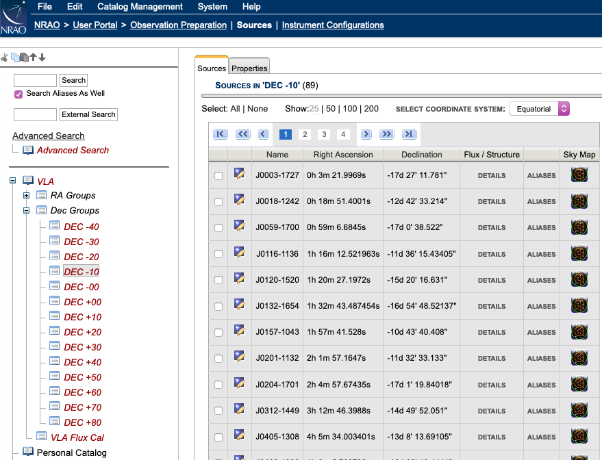
| Figure 2.1.2: The first few sources in the DEC -10 group, which is part of the Dec Groups in the VLA calibrator catalog. |
If you click on the catalog name, you will also see the contents of the highlighted VLA catalog in the main SCT window. This table list combines the contents of all groups and possible entries in the catalog that do not belong to a group (though in this case there are no such free-agent entries). The predefined groups in the VLA catalog are RA Groups, Dec Groups, and VLA Flux Cal. The RA Groups and Dec Groups also have subgroups (Figure 2.1.2), but these subgroups are a special case implementation in the VLA catalog only; groups cannot be nested. When a group name is highlighted (or selected) using the mouse button, the right-hand side window with the contents will only show the sources which were grouped in this sub-catalog. For example, selecting the VLA Flux Cal group will now only list the standard flux density calibrator sources. Similarly, the DEC +10 subgroup will show the VLA sources with Declinations between +10 and +20.
Clicking VLA differs from clicking the plus icon in that it will expose the total content of the catalog in the main (editing) window, with 25 sources per page, starting with source J0001+1914; clicking the plus icon only exposes the names of the groups in the left-hand side column. At the top of the table you will notice that the first line is a small page navigation menu; a similar page navigation menu can be found at the bottom. This VLA catalog contains more entries (currently showing 25) than fit on one page, and in this case is distributed over many pages. Below is a list of the menu icon buttons and a brief description:
| first page of the catalog (or group) | |
| 10 pages backward in the catalog (or group), or as many as possible if less than 10 exist | |
| previous page in the catalog (or group) | |
| 1, 2, .. | individual page numbers in the catalog (or group), with the current page highlighted click to select another page from this small list (up to 10 pages numbers) if desired |
| next page in the catalog (or group) | |
| 10 pages forward in the catalog (or group), or as many as possible if less than 10 remain | |
| last page of the catalog (or group) |
If you find the default of 25 lines per table page too few, you can change to a larger number of lines per page (50, 100, or 200) at the top of the page. Every table column with the font turning orange when the mouse hovers over it can be sorted by using a click of the mouse button. All pages in the catalog are used in the sorting which means that catalog entries may have moved from one page to another after a sort. When a column is sorted, it will show a small orange arrow next to the header name, pointing up if the column is sorted in ascending order (going to larger values when going down in the table) and pointing down when the sorting is in descending order. A sorted table can be re-sorted in the opposite direction by clicking the column again (note that the header of a sorted column, the one with the arrow, might not change to the orange color).
As a small exercise, use the navigation tools at the top or bottom to confirm that (with 25 sources per page) the catalog has 75 pages. Using the table header sort, confirm that the source with the most southern Declination is J1118-4634. Hovering the mouse over the Details or Aliases pops up, if available, additional information on the sources: flux densities at different frequency bands, closure phase properties, and aliases for the source in non-sortable columns (see the key in the VLA calibrator manual). The angular view near a calibrator on the sky can be displayed in a new browser tab by clicking the Sky Map icon  . Above the table on top of the page it is shown that the coordinates in the table are in the Equatorial coordinate system. If another coordinate system is selected in the drop-down menu, e.g., Galactic, the positions are recalculated from the positions entered originally, which is indicated by a small red asterisk next to the coordinates.
Each row in the table represents one source with a name and some descriptive information. A row starts with a tick-box and an edit icon  . The tick-boxes can be used to select one or more entries in the catalog for copy/paste as described in the next section. A shortcut to select all or to deselect all catalog entries on the current page can be found above the table. Selecting and copy/paste has to be redone for every page. The edit icon is used to access the details of the source entry in the catalog, i.e., the specifics of the source of interest. Here it will be a VLA calibrator source; later this might be the specifics of your science target source, and the information contained may be slightly different from entries in a personal source catalog created by an observer or by the PST to OPT import performed by NRAO staff.
Select a random source (not J1118-4634) and expose the source details by clicking on the editing icon in front of the name of the source of which you want to view the properties. The properties of the source are divided over three tabs in the main editing window labeled with the source's name, Images, and Notes. Most of the useful information is in the first tab labeled with the source's name: the source name and position. The Images tab holds the Elevation curve for this source, the LST times for different elevation limits that is useful for calculating LST ranges for which this source can be observed above a certain elevation, and the Azimuth curve. Another useful piece of information is in the Notes tab. Press the blue circle with the white triangle/arrow to show the VLA calibrator manual entry for this source (and press it again to hide this information). This and some extra information in a different form is given in the same tab under User Defined Values.
Navigate back to the VLA catalog either by clicking VLA in the catalog column tree, or by clicking Return to VLA (or, e.g., DEC +10, depending on how you got there) at the top of the page. Please allow the SCT to finish its operation and do not use the browser Back button.
Other read-only catalogs may contain or use slightly different source properties and auxiliary information. In particular, the source names are those of the original catalogs and not necessarily in accordance to the J2000 IAU convention as in the VLA catalog.
OPT 1.31 User Interface Updates
With version 1.31 some customization had been introduced to the SCT. These customization include the ability to resize the windows that make up the SCT (the left column tree structure display, the bottom warnings and errors display); the ability to change the size of the display fonts; and the ability to change the display color with several default themes. Note that these customizations will only be applied to the SCT; when you go to the RCT these customizations will go away. For example, if you are using a theme other than for Standard Light, when you go to the RCT the theme will reset to Standard Light. Going back to the SCT will reset to the custom theme.
Resizing Windows
New with OPT 1.31 is the ability to resize the left column tree structure display and the bottom warnings and errors display. To resize these windows move your cursor over to the inside long border of each window, click and hold on the border, and resize the window. Both windows do have a minimum size preset as the default size, therefore you can not completely close down the window.
Font Size
New with OPT 1.31 is the ability to reset the font size from the default. The options are for Large and Medium (see Figures 2.1.3.a-c below). Note that the alternative font sizes do not apply to the fonts in the top blue menu bar.
 |
| Figure 2.1.3.a: Default Font Size |
 |
| Figure 2.1.3.b: Medium Font Size |
 |
| Figure 2.1.3.c: Large Font Size |
Custom Themes
New with 1.31 is the ability to change the theme from the default Standard Light. The custom themes are: Standard Dark, Galaxy, Nebula, Star, Comet, and Asteroid. Examples of these theme colors are below (Figures 2.1.4.a-g). These themes are only available in the OPT and SCT and will not carry over to the RCT, which uses the default Standard Light theme.
 |
| Figure 2.1.4.a: Standard Light (black text on medium gray) |
 |
| Figure 2.1.4.b: Standard Dark (white text on dark gray) |
 |
| Figure 2.1.4.c: Galaxy (white text on blue-gray) |
 |
| Figure 2.1.4.d: Nebula (purple text on dark gray) |
 |
| Figure 2.1.4.e: Star (yellow text on dark gray) |
 |
| Figure 2.1.4.f: Comet (white text on blue-green) |
 |
| Figure 2.1.4.g: Asteroid (black text on teal) |
Create a Source Catalog
Overview
Personal (re)source catalogs can be created, modified, and removed using the menu strip and icon menu at the top of the tools page. It is convenient to collect (re)sources for a specific project in a separate catalog, especially for convenience during SB creation and also when sharing with co-I's.
For all approved VLA proposals submitted through the PST, once your project has been imported into the OPT by NRAO staff, a source catalog will be created and populated with the approved sources from the proposal. This source catalog will be labeled with the proposal/project code (e.g., 20A-123) and located in the left-hand side column. You should follow the exercise in the previous section and examples below to get a feel for what is in your source catalog. This is also a good time to double check the source coordinates of your science targets in your source catalog. How to modify the content will be explained in a later section.
Important Note: The OPT does not use global source properties; if you modify a source you must use the OPT to re-import the updated source to every applicable scan. For this procedure, a Bulk Scan Edit feature (described in a later section) has been implemented in the OPT per SB.
Icon Menu and Menu Strip Options: The icon menu is the line of little icons at the top of the (re)source catalogs in the left-hand side column. They have the same functionality as the options from the menu strip (below), although not every menu strip option is represented as they are not used as often. Only basic cut/copy/paste and reordering can be done with this icon menu. Note that the actions selected from the icon menu apply only to editing in the left-hand side column. Only valid actions will have an active icon in the menu, i.e., pasting an item may only be performed after copying or cutting the item first — until then the paste-icon will appear grayed-out. Hovering over an item with your mouse will display a pop-up tool-tip help to remind you of the action attached to the icon, but we also show them for reference below:
| Cut (or delete) selected tree item | |
| Copy selected tree item | |
| Paste selected tree item | |
| Move the selected catalog up in the tree | |
| Move the selected catalog down in the tree |
The same icon menu can be found in the RCT; for the OPT we will present additional icons for more options related to ordering scans in the OPT. Remember that these icons act only on the left-hand side column items.
The menu strip in the dark blue banner at the top of the page is used for creating new catalogs: FILE → CREATE NEW → CATALOG. It is not advisable to copy the VLA catalog into a new personal catalog and add new target sources, but it is useful to copy VLA sources into a new or existing personal catalog. The menu strip options under FILE and EDIT are grayed out with a line through them if that particular option is not valid for the current selection (highlighted item in the catalog tree in the left-hand side column). If the action you want to perform shows up as an invalid option (e.g., EDIT → CUT → GROUP to delete your group of sources) this usually means that you are not at the right place in the tree (e.g., not in the group, but in the upper level catalog). The names of the actions are self-explanatory, so we only list them for reference in the table. A similar list of menu strip options is available in the RCT and OPT, but with options specific to the tools. The menu strip options may act on both items in the left-hand side column as well as items in the main editing window.
| File |
Edit |
Help |
|---|---|---|
|
Create New → Catalog → Group → Source |
Cut → Catalog → Group → Sources |
About the SCT About Me Documentation Contact Support |
|
Export XML... Export PST... Import... Exit |
Copy → Catalog → Group → Sources |
|
|
|
Paste → Catalogs → Groups → Sources |
Add Sources to a Personal Catalog
There are three ways to add sources to a personal catalog, each described below. A fourth one is that the OPT gets filled with information from the PST once the TAC has approved observing time for your project. If you find a catalog imported directly from the PST, please carefully check the target source positions before you start using them in the OPT as you may have not entered them in the PST as you want them to appear in the SCT/OPT.
Import Source Lists
If you or a co-investigator uploaded a source list with your proposal in the PST, and this source list has not been transferred from the PST (or you prefer to delete that one), you should be able to get a head-start by uploading the same source list to the OPT. Use FILE → IMPORT... to communicate with a dialog box. Choose PST as input format and name your source catalog after it has been uploaded by selecting the New Catalog and navigating to the Properties tab. As a reminder, the PST format is/can be found in the relevant section of the PST manual (or in the complete description) in case you decide to make such a file at this stage. You may want to check the details of some sources to verify that the information has ended up correctly in the source property definitions. Verifying it now may save you more trouble later on when creating SBs.
If you would like to create a source list, the section, Text Files and Catalogs in the OPT Suite, describes in more detail the syntax, how to create a source list, and provides source list examples.
Copy Sources from Existing Catalogs
It is likely that your anticipated calibrator sources (which may not have been included in the proposal cover sheets) are already defined in the VLA calibrator source catalog. You can search for calibrator sources using the search tool described earlier in this section. In the catalog (or group) or in the search results you can select one or more sources you desire to add to your personal catalog by ticking the check-box(es) in front of the source name and editing icon using the top menu strip EDIT → COPY → SOURCES, etc. Then select the destination catalog or group and simply paste the copied sources: EDIT → PASTE → SOURCES, etc. You must repeat this action for each catalog or search results table page. Again verify that the source information in your personal source catalog is correct, e.g., by adding additional digits to a source position, prior to assigning source information to scans in the OPT. An example sequence would be as follows:
- Make sure you have navigated to the SCT.
- From the top menu strip select FILE → CREATE NEW → CATALOG; you can skip this and the next step if the catalog you want to use already exists and is writable (the catalog name is not in red italic font), e.g., the catalog automatically generated with your project ID.
- Your new catalog with the default name [New Catalog] appears in the main editing window, in the Properties tab. Change the name of the catalog to something useful to remind you of its purpose.
- Optionally, add the names of coauthors that you want to share the catalog with and who may edit the sources in the catalog.
- At this stage you may choose to group your sources. This is not necessary but convenient if you are going to have many sources. If you want to group sources in this catalog, select FILE → CREATE NEW → GROUP and name your group under the Properties tab.
- Click to navigate back to the first tab: Sources.
- Select the VLA source catalog and perform your source search as described previously; use Advanced Search or External Search if necessary.
- In the source table to the right, in the main editing window, check the source(s) you want. If you don't know which source to select, study the details of each before selecting one. If there are more sources than fit on a page you can change the number of sources per page from 25 to 50 or 100, or use multiple actions to select all your sources in subsequent steps.
- From the top menu strip select EDIT → COPY → SOURCES.
- Select your newly named source catalog (or group within it).
- From the top menu strip select EDIT → PASTE → SOURCES. If there are groups in the catalog, you will have the option to add them to a group as well. The sources now show up on the right-hand side.
- This can also be achieved by copy/paste of entire groups and/or entire catalogs using the top menu strip options or the menu icons at the top of the (left-hand side) source catalog column. Use the fly-over tool-tip help to identify the proper icon for each action.
- You may check the source properties using the Show/Edit icon for each catalog entry. You can also reorganize your sources by adding groups (FILE → CREATE NEW → GROUP) and move your sources around using the column icon menu, or using EDIT in the top menu strip. Unwanted sources can be deleted using Cut.
- If you are unhappy with the name of the catalog or group you can always rename it by selecting it and then clicking on the Properties tab.
Note that sources do not have to belong to a group. If you have specified groups, sources that do not belong to that group will not show up if you select that group. When there are sources in groups and sources not belonging to a group in the same catalog, you can only see and select a source without a group when you select the entire catalog.
Saving and Downloading Searches
With the upgrade to OTP 1.36, you now have the ability to save the search to a catalog in your Source Catalog database, or download the search as a text file, the contents of which can be uploaded to the Proposal Handling Tool.
Once you have performed a search and you have your results, if you click on the Save button (Figure 2.2.1) you will get a pop-up window asking you to set the name of the catalog (Figure 2.2.2). Enter the name of the catalog and click the Save button. In the left hand tree, a new catalog will be created with the name, and the contents of which will be the search results (Figure 2.2.3).
  |
| Figure 2.2.1: Saving the results of a search to a catalog. (Click to enlarge.) |
  |
| Figure 2.2.2: Pop-up window to name catalog. |
 |
| Figure 2.2.3: Search saved as catalog in your source catalog area. |
If the Download button is selected (Figure 2.2.4), the search results will be downloaded to your local computer. Some operating systems may allow you to select the directory / folder for the download and the name of the file; others, such as MacOX, will default to the Downloads folder and a default name of search_catalog.pst. The extension of .pst is so that this file can be uploaded to the Proposal Submission Tool, but it can cause issues in some operating systems as the extension .pst is unknown; the file itself is a plain text file, so just change the extension from .pst to .txt and you can view the contents with you favorite text editor (Figure 2.2.5).
 |
| Figure 2.2.4: Downloading the results of a search to local computer. (Click to enlarge.) |
 |
| Figure 2.2.5: Downloaded text file. (Click to enlarge.) |
Source Search
Select the VLA catalog in the catalog tree at the left-hand side and view the main editing window to the right. Source names follow J2000 IAU naming convention (i.e., truncated 10-character Jhhmm+ddmm) and aliases can be found by hovering over Aliases or by viewing the source properties (by clicking on the edit icon ). With the OPT 1.36 update, the B1950 Epoch has been disabled for all sources not currently using B1950, and for all sources added in the future; only Epoch J2000 should be used. To find source 3C279 it may take a while, even if you know this source is J1256-0547 (note the capital "J") in the IAU convention. Entering 3C279 (note the capital "C") in the source search tool in the upper part of the left-hand side column will search the selected source catalog for the source name in that catalog. If the "Search Aliases As Well" tick-box is not ticked, the search will only be matching for the name entered in the catalog (for VLA these are IAU names, but in your personal catalog you could have named your source 3C279 or "Skippy", etc); it then will only find this source in the VLA source catalog if J1256-0547 is entered. Therefore the aliases tick-box is by default ticked, but because searching is done on partial strings you may want to remove the option if you otherwise expect many matches (e.g., if you are looking for your source matching on the string "C" and don't want all 3C-sources to appear).
Because the search is performed on a partial string, searching for "-" (a minus sign) in the VLA catalog, for example, will return a 16 page table with all VLA calibrators with negative Declination (J2000), plus some extra sources with a minus sign in the name if you left the "Search Aliases" checked. A search on 1331+ will return 3C286 (as J1331+3030). Searches should not be case sensitive, but sometimes weird returns happen if lower cases are supplied; use upper case (J, B, C) for the standard VLA calibrators and their aliases. Two wild-cards are allowed: "?" and “*". They have the usual meaning of a single arbitrary character and any number of arbitrary characters, respectively. However, they are only useful between two other characters in the search string, as the search on *string* is automatically performed as a search on an empty search string which returns the entire catalog.
A source may also be obtained using the External Search if it is unknown to any of the existing catalogs. This search will be performed on the names, including aliases, in the SIMBAD database, using the same search and character rules.
Advanced Search
The Advanced Search (Figure 2.3.1) is used to search in an existing, selected catalog for other criteria than source name or alias. A common example is to search for a nearby calibrator at a position of your source of interest. This Advanced Search will bring up a dialog box in the main editing window containing various search parameter options. In that window, select the catalog(s) in which the search should be performed, and select the table(s) with the required parameters by checking the upper left tick-box of the relevant tables. Above the search parameter tables, you can select "All" or "None" catalogs and subsequently toggle individual catalogs. Table options and editing fields become active only when you select to use it. More than one catalog and more than one parameter table may be selected; the search interprets additional parameters as an AND condition. To perform the search, click the "Search" button below the parameter fields. Be patient, as searching can take a while; please do not continue clicking with the mouse button until the search operation has finished.
 |
|---|
| Figure 2.3.1: The various search parameters of Advanced Search. |
|
Advanced Search Parameters |
|
|---|---|
| Cone Search |
|
| Search By Calibrator Code |
|
| Search By Flux Density |
This parameter searches for flux densities above the given limit in the selected observing band. This is of course only useful when flux densities are included in the catalog(s) selected. |
| Search By Name |
This is the same search action with the same string rules as for the string entered in the top search tool in the left-hand side column, with the difference that here more than one catalog can be searched, and that other constraints can be included. |
|
Search By Right Ascension and Search By Declination |
Both are performed on a J2000 coordinate range, with the equal to or greater than (>=), or equal to or less than (<=) operators on the given limits. They use the same rules on entering positions as for the Cone Search. When both limits are given, the search returns the sources between the limits (i.e., you will see proper results for a search on sources with RA between 23 and 01 hours). |
Search Results
To submit the search parameters entered in the Advanced Search Parameters fields, click on the Search button. The sources matching the search parameters are listed below the Search Results header at the bottom (Figure 2.3.2). The results of a search are displayed read-only in the familiar SCT table format in a Search Results tree structure with the possibility to sort on different columns. Previous searches may be saved in the left-hand column tree for convenience — navigating to a previous search is done by simply selecting that search. Sources presented in the Search Results can be selected, and added to a personal source catalog using copy/paste, etc.. Search results are cleared when you log out of the SCT or the OPT Suite.
 |
| Figure 2.3.2: Advanced Search results using the Cone Search. This also shows the Flux / Structure information when hovering over DETAILS with a mouse. |
SCT 1.31 User Interface Update
Cone Search Sky Map
New with 1.31 is the ability to create a sky map based upon the cone search RA and Dec positions and search radius in degrees. This is accomplished by checking the catalog you wish to search in the list above the search parameters, then check on the Cone Search. Enter the RA, Dec, and search radius. Then click on the Search button to load the parameters into the Sky Map (Figure 2.3.3). Then click on the Sky Map icon in the Cone Search box to show the Sky Map (Figure 2.3.4).
|
Figure 2.3.3: Cone Search parameters for Sky Map |
 |
| Figure 2.3.4: Sky Map result with information for J0006-0004 (mouse hovering over source in map) |
Hide Catalogs
With 1.31 you have the ability to hide the catalogs that you find in your tree (left hand column) in order to help with organization. To do this, in the Menu do View → Hide/Unhide Catalogs (Figure 2.3.5). You will be presented with a list of your catalogs with check boxes. Select the catalogs that you want to hide by clicking in the corresponding box, then click on the Update button (Figure 2.3.6) Note that the catalogs will still appear at the top of the Search page, so they are not hidden from there.
|
Figure 2.3.5: Hide/Unhide menu option |
| Figure 2.3.6: List of catalogs to hide/unhide |
Create a New Source
If you do not use the PST upload file and your source does not appear in any of the existing catalogs, you will need to create a new source in a source catalog (or group) after selecting (or creating) the catalog or group you want to place the source in:
FILE → CREATE NEW → CATALOG/GROUP (if the catalog/group does not already exist)
FILE → CREATE NEW → SOURCE (in the desired catalog/group)
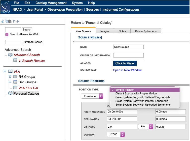
You will be presented with a blank source page consisting of four tabs labeled New Source, Images, Notes, and Pulsar Ephemeris (Figure 2.4.1). Name your source something convenient to search for at a later point, and fill in the necessary details (described below). You may also care to fill in the origin of your data for your own reference (e.g., PST file name, SIMBAD data base, etc.).
Source Positions
The SCT allows five different types of positions to be entered (Figure 2.4.1):
- Simple Position
- Distant source with Proper Motion
- Solar System Body with Table of Polynomials
- Solar System Body with Internal Ephemeris
- Solar System Body with Uploaded Ephemeris
By default the first option in the drop-down menu is Simple Position. Select a coordinate system (Equatorial, Galactic, or Ecliptic) and equinox (only J2000 should be used) in which you specify the coordinates and, if you care, also supply a distance (if known).
 |
|---|
| Figure 2.4.1: New Source information. |
If you select something other than Simple Position, the new selection will redraw the position table accordingly with all variables defaulted. You can select a predefined Solar System body name, upload an ephemeris table, or you can specify the position and some motion terms valid for some time range.
Motion terms are entered as polynomials, one for RA and a separate one for Dec, in time and are assumed to be representing the actual position for a certain time interval ("valid" box at the bottom):
position at Reference Time in Equinox + value(1) × time + value(2) × time2 + value(3) × time3, etc.
where the RA/Dec of the source at some point in time (defined in the "reference time" in the box below it) functions as the starting point of the polynomial. You would have to enter a "motion term" explicitly as, e.g., "3.4 x time - 0.5 x time2" (where "x time" may be abbreviated by "t", i.e., "3.4t - 0.5t2" and where "t2" is entered as "t^2"). Note that a value without a "t", "t2", etc, attached to the value will not be accepted. When imported as a source in a scheduling block in the OPT it should already show the position as for the date put in the reports tab; this will be updated at the time of actual observing. As the proper motion is given in actual angle (on a big circle), be aware that the motion in RA is calculated along the celestial equator, regardless of Dec, meaning that a proper motion in RA will yield the same RA-coordinate for a source at Dec=0d or e.g., Dec=60d. That is, there is no "cos(δ)" projection-term in the RA-coordinate change.
The motion term units and uncertainty will help recalculating the position (and error) at the time of observations, though this is currently not yet fully tested. Leave the motion terms blank if the source is considered not to move in the specified time interval. If you need another position and/or different motion terms for another time interval, simply add another time interval or add another source with a different name and position to the catalog and use it as appropriate. More information, in particular about generating ephemeris files, is given in the Observing Guide under Moving Objects.
Always double check the correctness of the source positions before searching for appropriate calibrators and before creating SBs.
Source Information
Images tab (Figure 2.4.2) displays the Visibility Chart consisting of the elevation and azimuth of the source as function of LST together with a table of rise and set LST (at 8° elevation) and some other elevation/azimuth and LST properties for your reference. Below are Image Links. It allows you to keep a catalog of image URL links, e.g., to the images in the VLA archive; use ADD or REMOVE SELECTED as many times as desired.
Notes tab is where you can collect all other information you wish to attach to this source. For example, for a target source you can remind yourself of the nearby calibrators you have found to be useful at some frequency, a reference to a paper mentioning an alternate position or a source property, or anything else you want to note. Click the blue expand button or New Note to add information to the Notes field. You can add links to papers or any other URLs for that matter. User defined values can be added at the bottom, e.g., the UV-range you determined to be proper for a point source calibration model, or whatever you deem useful.
Pulsar Ephemeris tab Certain VLA pulsar observing modes (binned imaging, and phased-array fold mod) require a pulse period ephemeris file be attached to the source. A Tempo-format ephemeris (also known as a "par file") for the source can be uploaded via this tab. Refer to the pulsar section in the VLA observing guide for more information.
 |
|---|
| Figure 2.4.2: Example of 3C286 Images tab in the SCT. |
Resource Catalog Tool
Introduction, Nomenclature, and Defaults
To access the Resource Catalog Tool (RCT), either login to the OPT Suite via the OPT (https://obs.vla.nrao.edu/opt) and select Instrument Configurations in the navigation strip, or you may use the following URL: https://obs.vla.nrao.edu/rct. Note, to exit the tool properly, use the Exit link in the upper right corner or log out with FILE → EXIT; do not close the browser window/tab until you are properly logged out of the tool.
On the left-hand column of the RCT, you will see an icon menu at the top, NRAO default catalogs along with an empty Personal Catalog you may populate, and possibly other catalog(s) (Figure 3.1.1). Note that an empty resource catalog for each of your successful proposals may be created. You may use this catalog to create personal resource setups or copy/paste NRAO default resources for easy access when creating SBs.
If you have any questions, you may either submit your questions through the NRAO Science Helpdesk or request help directly from the RCT by selecting HELP → CONTACT SUPPORT.
 |
|---|
| Figure 3.1.1: Left-hand column of RCT. |
Nomenclature
As per the SCT, for orientation and to get a feel for the tool(s), it is instructive to walk through the NRAO Defaults catalog. After this orientation it should be almost intuitive to create your own personal resource catalog(s) which you will use in your project's SB scans or help to understand how to use one of the standard wide band resources provided in the NRAO Defaults catalog.
Important Note: Data from the WIDAR correlator is different from the old VLA correlator: the data is always delivered in spectral line or pseudo-continuum mode, similar to Very Long Baseline Interferometry (VLBI). When referring to continuum below, it is meant to refer to data taken for wide band observation purposes: the data itself is divided in frequency channels, but the scientific interest is in the data averaged over all channels and not in individual channels with line emission (or absorption). The latter is referred to as spectral line data. This is the difference in obtaining a two-dimensional image of the sky versus a three-dimensional image cube, where the data retains that different frequencies show different (two-dimensional) sky images.
The best continuum sensitivity is obtained using the maximum available bandwidth in the most sensitive part of the observing band, and thereby avoiding Radio Frequency Interference (RFI) as much as possible. The resource which gives the best performance in each observing band is defined in the NRAO Defaults catalog. To describe the setups, is it useful to understand how the basic generalized path of the radio frequency (RF) signals collected by the receivers in the antenna are delivered through the intermediate frequency (IF) electronics to the WIDAR correlator and where the correlated data ends up in a data set.
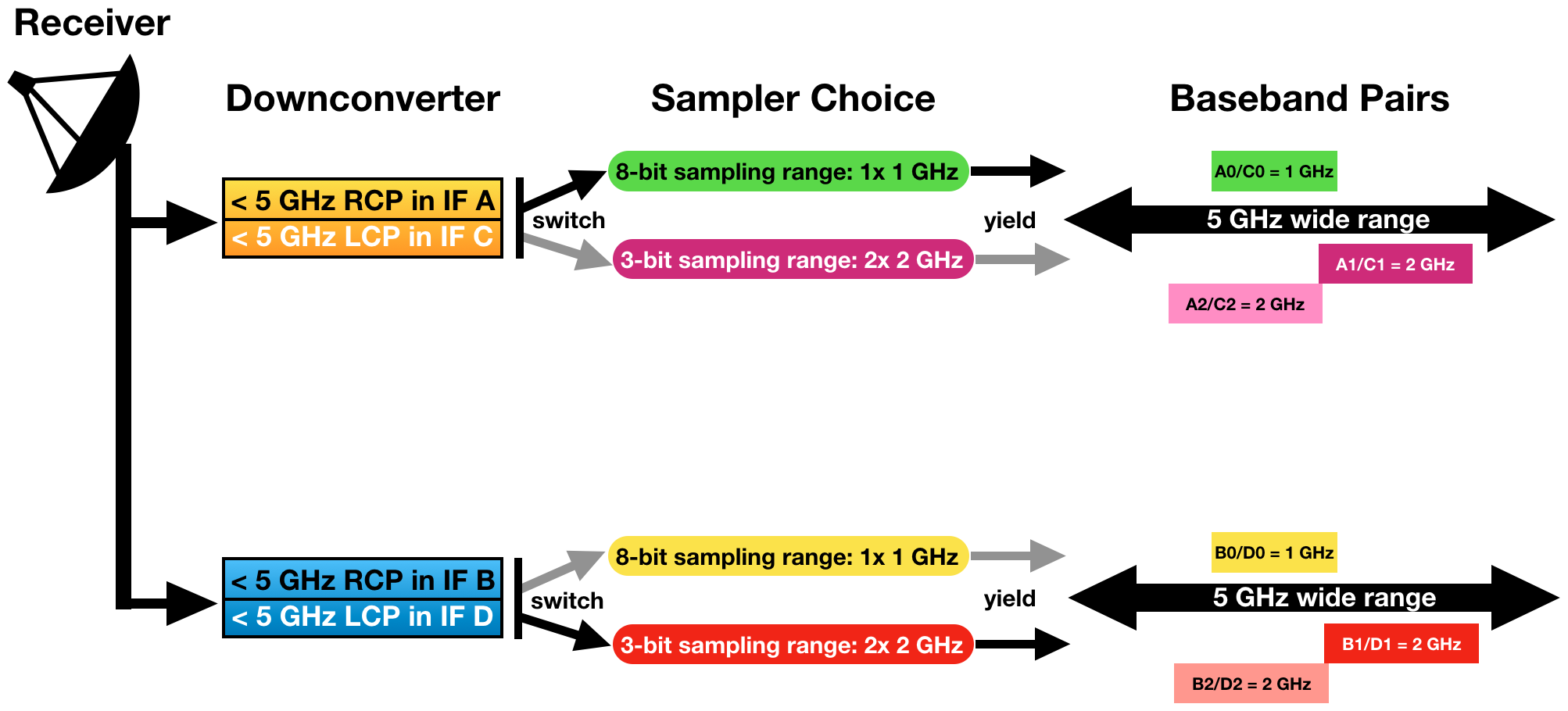
Baseband Pairs
The receiver in the antenna passes (up to) 5 GHz down-converted frequency of the RF receiver bandwidth to four signal paths (Figure 3.1.2); two right circular polarization signals (RCP), labeled IF A and IF B, and two left circular polarization signals (LCP), labeled IF C and IF D. IF A and IF C (i.e., one RCP and one LCP) signals are tuned to the same RF frequency and thus may produce a Stokes I signal from the source. IF B and IF D are also tuned to the same frequency, which typically is not the same tuning as for IF A and IF C. These IF signals are then sampled independently using 8-bit samplers or 3-bit samplers. The VLA Samplers section of the OSS should aid in which sampler to use for your observations. The 8-bit samplers each yield a one 1 GHz wide frequency range containing a corresponding 1 GHz down-converted RF range. The 3-bit samplers each yield two 2 GHz wide frequency ranges containing two corresponding 2 GHz down-converted RF ranges. Per IF path (AC or BD) the two 2 GHz ranges from the 3-bit samplers must be within a total range of 5 GHz and are typically placed to yield a continuous 4 GHz RF bandwidth per IF path, or an 8 GHz RF bandwidth total.
The individual sampled frequency ranges are referred to as basebands, in particular baseband pairs when a combination of simultaneously tuned RCP and LCP signals is involved. The 8-bit samplers yield 1 GHz baseband pairs which are labeled A0/C0 or B0/D0, depending on the original IF path. The 3-bit samplers produce 2 GHz baseband pairs labeled A1/C1 and A2/C2 as sampled from IF path AC, or B1/D1 and B1/D1 if the signals are sampled from IF path BD. These baseband pairs are then transported over optical fiber from the antennas to the correlator.
Part of setting up the resource is to specify which samplers are used and to specify the baseband pair center sky frequencies.
 |
|---|
| Figure 3.1.2: Schematic of nomenclature and the involvement of the 8-bit and/or 3-bit samplers. |
Subband Pairs
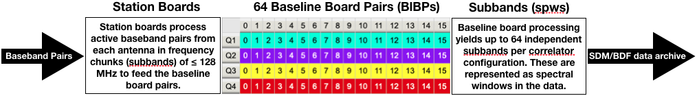
When the basebands from each antenna reach the correlator room, they are fed in 128 MHz bandwidth intervals into station boards. This regular pattern of 128 MHz creates a fundamental interval boundary which cannot be observed, nor included in processing of nearby frequencies. Apart from the baseband edges, there are 7 of such un-observable frequency boundaries per 1 GHz (1024 MHz) baseband when using the 8-bit sampler, and 15 per 3-bit sampler baseband (i.e., per 2 GHz, per 2048 MHz). Note that since this is an odd number, the chosen baseband center sky frequency can never be observed: do not place the baseband center at the frequency of your spectral line. From each 128 MHz chunk, the station boards determine which part (central frequency and frequency width) is forwarded to the correlator for processing. That is, per polarization for each 128 MHz bandwidth, it is determined whether the signal should be forwarded to the correlator, and whether each 128 MHz bandwidth should be divided in powers of 2 and tuned to another center frequency within the 128 MHz range: provided that the frequency interval does not cross the boundary when forwarded to the correlator.
The filtered and tuned frequency ranges delivered by the station boards are referred to as subbands, in particular subband pairs for simultaneously tuned RCP and LCP signals. The individual subbands are at most 128 MHz wide, and independently tunable in frequency if reduced in width by powers of two without crossing the 128 MHz boundaries. Per resource, up to 64 subband pairs can be defined.
Part of setting up the resource is to specify the frequency tuning and frequency width of the subbands that are to be used.
Baseline Board Pairs (BlBPs)
The resulting subband pairs per antenna and IF path are presented to one of the four correlator quadrants for processing by pieces of hardware known as baseline boards, or baseline board pairs (BlBPs) when the subband contains both RCP and LCP signals. Figure 3.1.3 (below) is a simple visualization of the correlator components. Up to 64 BlBPs process the baseband pair streams from the antennas as formatted by the station boards in four quadrants (Q1-Q4) with 16 BlBPs per correlator quadrant. A single BlBP can only receive data from a single subband for processing. Per BlBP 256 correlation products can be computed, where the number of products is the number of polarization products (1, 2, or 4) times the number of spectral frequency points (256, 128, or 64). Within the limits of the number of baseline boards in a correlator quadrant, more than one baseline board can be assigned to process a single subband pair (thus up to 16) at the cost of processing other subband pairs.
A resource defines the output of the station boards (after defining the baseband pairs at the antennas) and the assignment of the available BlBPs for processing to yield up to 64 independently configurable subbands with spectra. These subbands will end up as a simultaneously observed subset of spectral windows (spws) in the visibility data. At most, one subband (of 128 MHz or less bandwidth) can be processed per BlBP, but more than one BlBP can be used to process the same subband (called baseline board stacking), yielding a larger number of channels to obtain an increased spectral resolution over the bandwidth of that subband (in the case without recirculation). In other words, baseline board stacking utilized by assigning more than one baseline board to a single subband. Without recirculation, the combination of subband width, number of polarization products and number of baseline boards determine the channel frequency width of the data in the subband. The OSS contains more details about the WIDAR correlator.
Part of setting up the resource is to specify the distribution of the computing power of the BlBPs over the active subbands.
 |
|---|
| Figure 3.1.3: Simplified schematic of correlator components. |
Spectral Windows and SDM/BDF
The correlated data consists of up to 64 independently tunable (center frequency and frequency width) and configurable (polarization and spectral frequency points) subbands per observing resource. This data is written as Binary Data Format (BDF) files to the archive, together with header and auxiliary information defining the corresponding Science Data Model (SDM) for the observation. Multiple resources can be used during an observation, and therefore many more than 64 subbands can be in the data; subbands contained in the SDM/BDF are called individual spectral windows (spws) in CASA (or IFs in AIPS). CASA can process non-homogeneously configured spectral windows simultaneously, but care must be taken in the interpretation of spws versus subbands when referring to an observing resource: any resource can have up to 16 or 64 subbands (for 8-bit and 3-bit respectively) but a data set may contain hundreds of spws (from multiple resources).
NRAO Defaults
The NRAO Defaults catalog (Figure 3.1.4) is a collection of hardware and instrument configurations (front-end receivers, correlator integration time plus observing/subband bandwidth and frequency channels, frequency tuning, etc.). They are expected to be good standards for wide band continuum observations using the VLA.
The NRAO Defaults catalog is in red italics (indicating read-only) and has a plus-icon in front of it (indicating groups within). If you click the plus-icon () or NRAO Defaults these groups will appear in the catalog tree. Similarly, clicking NRAO Defaults differs from clicking the plus-icon in that it will expose the total content of the catalog in the main window, with 25 sources per page, starting with a pointing resource group.
 |
|---|
| Figure 3.1.4: A snapshot of the NRAO Defaults catalog. |
Pre-defined resource groups in the NRAO Defaults catalog are Pointing setups and either 3-bit or 8-bit dependent groups. When a group is highlighted or selected using the mouse button, the right-hand side window with the contents will only show (filter) the resources which were grouped in this sub-catalog. For example, selecting the "up to 2x1GHz (8bit)" group will now only list the NRAO default resources using the 8-bit system. Similarly, the Pointing setups will show the NRAO default resources for pointing scans in C and X-band.
Note on reference pointing: Only the default X-band pointing resource (X-point) should be used for the reference pointing (interferometric pointing) scans. For how, when, and why to use reference pointing scans, refer to the Calibration section of the VLA Observing Guide.
Each line in the table represents one resource with a name and some descriptive information. A line starts with a tick-box and an edit icon (). The tick-boxes can be used to select one or more entries in the catalog for copy/paste as described in the SCT catalog chapter. Selecting and copy/paste has to be redone for every page. The edit icon is used to access the details of the resource entry in the catalog, i.e., the specifics of the resource of interest. Here it will be a NRAO default resource, but later this might as well be the specifics of your scientific target resource, and the information contained in these entries therefore may be slightly different from entries in a personal source catalog created by an observer.
Click NRAO Defaults in the left-hand side column to return to the NRAO Defaults catalog. The basic catalog rules, use of icons, browsing, table viewing, and the mechanics of creating and editing of resource catalogs is almost identical to that of the SCT. So to access the details of a single resource, click the edit icon ().
Wide Band Continuum Resources
Continuum observations are generally performed using the maximum available bandwidth to obtain the best signal to noise ratio for a signal that is (mostly) independent on frequency. The receivers for the upper three receiver bands (> 18 GHz: K, Ka, Q) cover more than 8 GHz bandwidth. To obtain maximum instantaneous sensitivity it is therefore possible, with the 3-bit samplers, to observe a full 8-GHz wide bandwidth for continuum purposes. On the other hand, signals obtained with the lower frequency receivers, where RFI is apparent and the receiver coverage is less than 4 GHz, are better sampled with the 8-bit samplers covering up to 2 GHz bandwidth. For C, X and Ku bands, one has to choose. Below, examples of a 3-bit and an 8-bit sampler default wide band resource are shown.
High Frequency
8 GHz Wide Band Continuum (3-bit, Ku, K, Ka, and Q-band)
As an example of a 3-bit wide band continuum resource, select the K64f3DCB resource in the NRAO Defaults catalog (in group "up to 4x2GHz (3bit)"). Click on the () edit icon (with fly-over help tool-tip Show/Edit properties for this catalog entry) to see the hardware and instrument options used in this resource.
The information displayed (Figure 3.1.5) in the top graphic is the receiver band coverage, one color per IF path, four in total. Furthermore the nominal (green, 1dB sensitivity drop) and extreme (white, 3dB) receiver coverage ranges are shown as vertical dashed lines. Two small tables show the Basics of the receiver (name and correlator integration time) and a summary of correlator resources used for this setup, which will update when further specifications are made. Note that this non-editable default resource uses the maximum of 64 BlBPs to cover 8 GHz of bandwidth within the allowed data rate. Below the graphic is a window with five tabs: Basebands, Subbands, Special Modes, Validation, and Comments.
 |
|---|
| Figure 3.1.5: NRAO Default K-band 3-bit resource. |
- Basebands tab summarizes the samplers in use and the central sky frequency to which each of the four (2 AC + 2 BD) 2-GHz wide baseband pairs are tuned, with their individual sky range bandwidths.
- Subbands tab lists, for each baseband under a different tab, the subbands as configured for the baseband. In this case there are 16 subbands of 128 MHz per baseband, each distributed over a single correlator quadrant (displayed by different colors, see also at the bottom of the Validation tab). Each subband will yield 64 spectral frequency points at full polarization. This setup thus will generate 64 spectral windows in the data; each 128 MHz wide divided in 64 2-MHz wide channels and 4 polarization products.
- Special Modes tab will indicate if RFI blanking has been enabled for this default resource.
- Validation tab summarizes the setup in receiver band and correlator integration time, baseband properties in the next table, and subband properties. Note that because the "yellow" baseband is centered at 19.000 GHz, and the baseband is not 2.0 GHz wide, but slightly wider at 2048 MHz, some (24 MHz) of the baseband is actually below the official 1dB limit of 18.0 GHz. This generates a warning, but in practice is not as serious as it appears.
- Comments tab will contain any comments regarding the resource setup.
Navigate back to the NRAO Defaults catalog either by clicking NRAO Defaults in the catalog column tree, or by clicking Return to NRAO Defaults(or up to 4x2GHz (3-bit), depending on how you got there) at the top of the page. Please allow the web application to finish its operation and do not use the browser back button.
Low Frequency
1 and 2 GHz Wide Band Continuum (8-bit, P, L, S, C, and X-band)
As an example of an 8-bit wide band continuum resource, open the S16f2A resource in the NRAO Defaults catalog (in group "up to 2x1GHz (8-bit)") (see Figure 3.1.6). The information in Figure 3.1.6 shows only two colors, one per IF path. This is a direct result from choosing the 8-bit sampler in the Basebands tab. The number of BlBPs used in this setup is only 16 to cover 2 GHz of bandwidth. The Basebands tab lists two (1 AC + 1 BD) 1-GHz wide baseband pairs with their tuning centered in S-band. Through the Subbands tab, and the tabs per baseband it is seen that there are 8 subbands of 128 MHz per baseband, each distributed only partly over the available correlator quadrants (per color used) to yield 64 full polarization spectral frequency points. This setup generates 16 subbands (or spws) in the data, the number of colored items in the correlator quadrant summary under the Validation tab. The subbands are 128 MHz wide divided in 2-MHz wide channels.
In addition to the 8-bit continuum resources for C and X-band, 3-bit continuum resources are also available.
 |
|---|
| Figure 3.1.6: NRAO Default S-band 8-bit resource. |
realfast
The default resources for L, S, C, and X-band are setup to use the realfast system. This is a commensal observing system that searches VLA data for millisecond-timescale dispersed transient signals in real-time, in parallel with normal VLA observations. For more details, visit the realfast webpage.
Spectral Line Observations
There is no separate example of a spectral line resource in the NRAO Defaults catalog. The WIDAR correlator writes all its data in spectral line format, meaning that the continuum resources described above are already spectral line resources with 2 MHz frequency channels. However, when the scientific interest is in a specific line, typically one would want to use a spectral resolution that is better than the 2 MHz channel width in the continuum resources above. The correlator would be set up to provide data with narrower frequency channels than 2 MHz, tuned to the line frequency when corrected for (approximate) Doppler shift. Note that the channel frequency width is not the final spectral resolution in the data cube as this depends on the actual data processing and whether, e.g., Hanning smoothing was applied in post processing. Smoothing will decrease the spectral resolution in the data. When planning on smoothing, be aware that the channel width only approximates the best spectral resolution available without smoothing, at about 1.2 times the individual channel separation. To get a particular spectral resolution with Hanning smoothing make sure that the line is oversampled with at least a factor of two (i.e., double the number of channels that you need for that spectral resolution). There are four possibilities to reduce the width of the frequency channels to obtain frequency channels narrower than 2 MHz for spectral line work; they can be used independently or simultaneously.
- The number of polarization products may be reduced from 4 to 2 or 1 to obtain contiguous 128 MHz subbands with a spectral channel separation of 1 or 0.5 MHz respectively.
- The subband bandwidth of 128 MHz can be reduced in factors of two to obtain factors of two narrower channel separations in that subband.
- When the subband bandwidth is reduced, processing capacity becomes available to process more lags. This is known as recirculation. The product of bandwidth and recirculation factor should be less than 128 MHz per subband.
- Processing of fewer subbands than the maximum of 64 allows the use of additional BlBPs to produce more channels. This is known as baseline board stacking.
For more information, refer to the Spectral Line section of the VLA Observing Guide and the WIDAR section of the OSS. The Spectral Line Setup section of this manual will describe how to setup a spectral line resource.
Create a New Resource Catalog
Overview
New resource catalogs can be created, modified, and removed using the menu strip and icon menu at the top of the tools page. It is convenient to collect resources for a specific project in a separate catalog, especially for convenience during SB creation and also when sharing with co-I's.
For all approved VLA proposals submitted through the PST, once your project has been imported into the OPT by NRAO staff, an empty resource catalog will be created. It is the responsibility of the observer to populate the resource catalog. This resource catalog will be labeled with the proposal/project code (e.g., 20A-123) and located in the left-hand side column.
Important Note: The OPT does not use global resource properties; if you modify a resource you must use the OPT to re-import the updated resource to every applicable scan. For this procedure, a Bulk Scan Edit feature (described in a later section) has been implemented in the OPT per SB.
Icon Menu and Menu Strip Options
The icon menu is the line of little icons at the top of the (re)source catalogs in the left-hand side column. They have the same functionality as the options from the menu strip (below), although not every menu strip option is represented as they are not used as often. Only basic cut/copy/paste and reordering can be done with this icon menu. Note that the actions selected from the icon menu apply only to editing in the left-hand side column. Only valid actions will have an active icon in the menu, i.e., pasting an item may only be performed after copying or cutting the item first — until then the paste-icon will appear grayed-out. Hovering over an item with your mouse will display a pop-up tool-tip help to remind you of the action attached to the icon, but we also show them for reference below:
| Cut (or delete) selected tree item | |
| Copy selected tree item | |
| Paste selected tree item | |
| Move the selected catalog up in the tree | |
| Move the selected catalog down in the tree |
The same icon menu can be found in the SCT; for the OPT we will present additional icons for more options related to ordering scans in the OPT. Remember that these icons act only on the left-hand side column items.
The menu strip in the dark blue banner at the top of the page is used for creating new catalogs: FILE → CREATE NEW → CATALOG. It is not advisable to copy the NRAO Defaults catalog into a new personal catalog and add new resources, but it is useful to copy individual NRAO default setups into a new or existing personal catalog. The menu strip options under FILE and EDIT are grayed out with a line through them if that particular option is not valid for the current selection (highlighted item in the catalog tree in the left-hand side column). If the action you want to perform shows up as an invalid option (e.g., EDIT → CUT → GROUP to delete your group of resources) this usually means that you are not at the right place in the tree (e.g., not in the group, but in the upper level catalog). The names of the actions are self-explanatory, so we only list them for reference in the table; the ones in square brackets only appear when relevant, in particular when a resource in a group is selected. A similar list of menu strip options is available in the SCT and OPT, but with options specific to the tools. The menu strip options may act on both items in the left-hand side column as well as items in the main editing window.
| File | Edit | Help |
|---|---|---|
|
Create New → Catalog → Group → Instrument Configuration
|
Cut → Catalog → Group → Instrument Cfgs. |
About the RCT About Me New Features Documentation Contact Support |
|
Export Catalog... Import Catalog... Import Resource... Exit |
Copy → Catalog → Group → Instrument Cfgs. |
|
|
Paste → Catalogs → Groups → Instrument Cfgs. |
Create a Personal Resource Catalog
If you would like to create a personal resource catalog and/or group within the catalog, take the following steps:
- Make sure you have navigated to the RCT.
- From the top menu strip select FILE → CREATE NEW → CATALOG.
- Your new catalog with the default name [New Catalog] appears in the main editing window, in the Properties tab. Change the name of the catalog to something useful to remind you of its purpose.
- Optionally, add the names of coauthors that you want to share the catalog with so they may view and edit the resources in the catalog.
- At this stage you may choose to group your resources. This is not necessary but convenient if you are going to have many resources. If you want to group resources in this catalog, select FILE → CREATE NEW → GROUP and name your group under the Properties tab.
- Click to navigate back to the first tab: Resources.
- If you are unhappy with the name of the catalog or group you can always rename it by highlighting it and then clicking on the Properties tab.
Note that resources do not have to belong to a group. If you have specified groups, resources that do not belong to that group will not show up if you select that group. When there are resources in groups and resources not belonging to a group in the same catalog, you can only see and select a resource without a group when you select the entire catalog.
Populate a Resource Catalog
Copy/Paste NRAO Defaults
Note: Due to changes/updates in the RCT on 2021 February 04, the NRAO defaults are not editable after copy/pasting to a personal catalog.
If your observations can use one or more of the NRAO Default (wide band continuum) resources, or you would like to use an NRAO Default as a template, it is advisable to copy/paste those default resources into a personal catalog. This will allow for an easier and faster process of creating SBs. To copy/paste one or more resources, take the following steps:
- Go to the NRAO Defaults catalog level. Note, if you go to a group level, e.g., DCB/Any Config, you will not be able to copy/paste a single resource, only the entire group.
- Select the resource(s) appropriate for your observations, then select FILE → COPY → INSTRUMENT CFGS..
- Go to the personal catalog (or group within the catalog) you wish to paste the resources into, then select FILE → PASTE → INSTRUMENT CFGS..
Recirculation vs Baseline Board Pairs
Creating a spectral line resource is similar to creating wide band resources as outlined in the previous section, except for the more advanced specification of the subbands and subband frequency tuning and possible Doppler setting of the frequencies. Eventually, resources with the requested correlator settings will be pre-filled from information submitted to the PST during the observing time allocation procedure. However, at this stage none of this has been implemented.
For how and when to use this observing mode, refer to the Spectral Line section of the VLA Observing Guide.
The NRAO Defaults resource catalog contains full polarization dual IF pair spectra-polarimetry resources (the wide band continuum resources). If they appeal to you, you can copy/paste them in a personal catalog just as for the wide band resources above and edit them as needed. Check the spectral line resource properties very carefully as the spectral line resources in the NRAO Defaults have a fixed sky frequency whereas you probably want to use a rest frequency in combination with Doppler setting. Most likely, however, you will opt to create your own resource, just like creating a wide band resource previously. Some items that need extra attention are described below, but first a small detour to outline the options for creating large numbers of narrow frequency channels.
Recirculation vs. Baseline Board Stacking
Spectral line observations are typically constrained by the requirement to have the best spectral resolution (i.e., narrowest spectral channel width) combined with the best velocity coverage (i.e., widest observing bandwidth), the latter perhaps also for calibration purposes (as gain calibration is done per subband).
The maximum subband bandwidth is 128 MHz and can be decreased by factors of 2 to 31.25 kHz(*). Total bandwidths wider than 128 MHz are achieved by placing subsequent bandwidths next to each other with the caveat that the few channels next to a subband edge should be considered lost for line work (on either side of the boundary, for continuum work as well). To obtain a contiguous bandwidth which is near-homogeneous in sensitivity and without any subband boundary gaps, another baseband would be placed some MHz offset (e.g., half a subband bandwidth) from the original baseband to enable subband stitching in post-processing. Note that this limits the number of available basebands for other line settings.
A single Baseline Board Pair (BlBP), out of 64 available BlBPs, can handle 256 spectral points divided over the polarization products (polProd). That is, it can deliver 256 spectral channels in single polarization, 128 spectral channels in dual polarization, or 64 spectral channels in full polarization. The channel width (which is slightly less than the spectral resolution) is then simply the subband width divided by the number of spectral channels.
With one BlBP per subband as standard, the selected subband bandwidth is thus limited to 256/polProd channels which may not be narrow enough to achieve the desired spectral resolution. There are two ways to overcome this limitation: Baseline Board Stacking uses more of the limited amount of hardware and Recirculation uses limiting the total bandwidth per subband and CPU cycles. Both have their disadvantages and the choice depends on the science requirements. If either can be used, we recommend using Recirculation.
Baseline Board Stacking uses additional BlBPs to compute extra channels in a subband (of any width up to 128 MHz). Each additional BlBP increases the number of spectral channels by 256/polProd. As there are only 64 BlBPs total, and as every subband uses a minimum of one BlBP, Baseline Board Stacking reduces the number of subbands that can be observed to less than 64, and in the extreme case to a single subband of 128 MHz or less. When most of the 64 BlBPs are being used and all of the subbands are required (instead of some being recognized as less important and thus "desired" versus "required"), the observations will not take place if one or more BlBPs are inoperable. The 3-bit NRAO default setups use 64 BlBPs with the subbands at the baseband edges "desired" to allow continuation of operations when not all BlBPs are available.
The Recirculation option uses software to compute extra channels. For this, CPU cycles are "freed up" by limiting the subband bandwidth fed to the BlBP to less than 128 MHz to obtain more lags (in factors of two), running the data through the board for a second, third, etc., time; hence Recirculation. As subband bandwidths (and CPU cycles needed to process them) can be decreased by factors of 2, each halving thus allows a doubling of the number of channels in the subband, currently up to a factor of 64. This does not require additional BlBP hardware and thus retains the possibility of using all subbands, albeit at less subband and less total bandwidth. Currently, subbands of 128 MHz must use Baseline Board Stacking to achieve more than 256/polProd channels.
Baseline Board Stacking and Recirculation can be used simultaneously in the same subband (if less than 128 MHz), and configurations with multiple subbands configured with either or both are allowed. Note that here a correlator setup can still request all 64 BlBPs and thus designating some subbands as "desired" is still highly recommended, but Recirculation gives the option to use less than 64 to achieve the number of spectral channels. However, requesting a large number of channels, whether or not with Baseline Board Stacking and/or Recirculation, yields higher data rates than normal with the default integration times. To remain within the limits set by the observatory, longer integration may be needed which has an impact on time averaging smearing in the larger array configurations and thus on the field of view.
The choice for one or the other, or even for less channels than anticipated, depends on the trade-offs that can be made for the science goals and remain a responsibility of the observer.
(*) When observing at such narrow subband bandwidths it is good to check with the NRAO Science helpdesk. There are other operational constraints, in particular the F-shift in bringing down the baseband, that need to be considered and that may decrease the usable subband bandwidth to much more than a (symmetric) few channels compared to the general case described above.
Custom Type Spectral Line Setup
On November 8, 2023, a new Resource Catalog Tool was introduced which changes the way custom resources are created. This section will cover the creation of a custom spectral line resource. If you have questions or issues, please contact us through the NRAO Science Helpdesk.
Create a Spectral Line Resource
After choosing to create a new instrument configuration, the New Resource Wizard pop-up box will appear with several options.
To create a spectral line resource select:
- Spectral Line
- Array Configuration: This will set the recommended default correlator integration time, which can be changed later in the tool if desired.
- Name: This should match the name of the resource entered in the PST.
- Finally, select the Generate button.
Basics Table
Near the top you will find the Basics info table (Figure 3.3.3a) which is common across all tabs. This is where you can change the name of the resource and the correlator integration time.
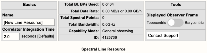 |
|
Figure 3.3.3a: Spectral line Basics info table. |
Below is a description of the parameters in the Basics table.
| Name |
Be sure to use unique names for all different resource setups and do not use special characters. |
| Correlator Integration Time (seconds) |
The correlator integration time would have been set when the resource was initially created by selecting one of the array configurations. This can be modified in the table if you do not wish to use a default setting. For more details, refer to the Time Resolution and Data Rates section of the Observational Status Summary (OSS). |
| Total Bl.BPs Used |
This indicates the total baseline board pairs used, i.e., correlator resources. The starting number will always be zero and will increase as lines and continuum subbands are added and when more baseline board pairs are used per line. |
| Total Data Rate |
The data rate of the resource will increase as lines and continuum subbands are added. Keep in mind the minimum and maximum data rates: Time Resolution and Data Rates. |
| Total Spectral Points |
The total spectral points will increase as the number of requested BlBPs increases. For a more detailed explanation, refer to the Spectral Line Resources section of the OPT manual. |
| Total Bandwidth (GHz) |
This will display the sum of all subband bandwidths across all basebands in GHz. |
| Capability Mode |
The will display the capability mode of a resource, e.g., general, shared risk, or resident shared risk observing. This will depend on the total data rate and certain other settings described in the OSS. |
| ID |
This is the resource ID. |
| Displayed Observer Frame |
Default is Topocentric (rest frame is the telescope and is what the VLA uses at the time of observing). This can be toggled to Barycentric (rest frame is Earth+Sun center of mass). |
| Contact Support |
Selecting this button will allow you to contact the NRAO Science Helpdesk. |
Doppler Position Tab
You must enter the coordinates of the science target (or near a grouping of science targets) in RA and Dec. This will unlock the proceeding tabs so you may continue with the creation of the resource. You can also import the RA and Dec from a source in your Source catalog.
Lines Tab
In the Lines tab, you may either enter in the line information one-at-a-time by selecting Add Line or import a text file containing a list of lines by selecting:
Import Spectral Lines → Browse (select the txt file containing the lines you want to import/upload) → Upload → Done (if using Firefox)
(Note, if you are using Firefox you will be required to select the Done button after selecting Upload to complete the import. It has been determined that other browsers such as Safari (Mac), Opera (Linux / Mac / Windows), Chrome (Linux / Mac / Windows), or Microsoft Edge (Windows) do not need the Done button to be selected to complete the upload.)
Example of a spectral line added to the Lines tab can be seen in Figure 3.3.3b.
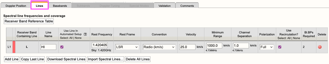 |
|
Figure 3.3.3b: Example of a spectral line added to the Lines tab. |
For each line you will need to provide the following information:
| Line Name |
Do not use special characters and keep the name relatively short. |
| Use Line in Automated Setup (all/none) |
You may choose which lines are used in the automated setup. This means you can upload a set of lines and only use some of them or use this option as a way to partially automate/manually setup your resource. |
| Rest Frequency |
Rest frequency of the line you wish to observe in GHz. |
| Rest Frame |
LSR, Topocentric, Barycentric, Geocentric |
| Convention |
Radio (km/s), Optical (km/s), Redshift (Z), Relativistic (km/s) |
| Velocity (km/s) |
The line-of-sight velocity at which the line should be observed. |
| Minimum Range (km/s) |
Specify the minimum velocity range that should be covered. Note that a first order bandwidth for this range will be calculated using the line frequency and displayed below the input field. This will set the subband bandwidth to the next wider possible value. Try to keep the bandwidth for the range as narrow as possible for your science to maximize flexibility in placing the 128 MHz boundaries between your anticipated subbands; you can widen them later. In general pre-defining subbands wider than 32 MHz will often give problems in the initial placing of the subbands. |
| Channel Separation (km/s) |
The (maximum) channel separation input field will display the velocity width converted to frequency below the input field, and set the channel separation in the subband to the next possible narrower value. |
| Polarization |
Full, Dual, Right, Left |
| Use Recirculation? |
Enabled is recommended. |
| Bl.BPs (baseline board pairs) Required |
This will auto-update as the other line information is entered. |
Below is an example of a line text file for a Spectral Line resource. For more details, refer to the OPT manual. You may also export a set of lines from an existing resource.
#Line name; Rest frequency; Rest frame; Velocity convention; Velocity; Minimum range; Channel separation; Polarization products; Additional specifications
L1; 38.293GHz; Lsr Kinematic; Radio; -10.5km/s; 31.0km/s; 0.01km/s; DUAL; USE_RECIRCULATION=true
L2; 38.452629GHz; Lsr Kinematic; Radio; -10.5km/s; 31.0km/s; 0.01km/s; DUAL; USE_RECIRCULATION=true
Basebands Tab
There are two options for generating the spectral lines in their respective basebands, automated and manual.
Automated Setup
This will automatically generate the line coverage in their respective subbands and properly center the basebands. Only one receiver band will be activated when your lines are spread over frequencies spanning more than one band.
- If all your lines fall below 4 GHz, i.e., up to the S-band frequency range, you will only be permitted to use the 8-bit system.
- If all your lines fall within the 4-50 GHz frequency range, the RCT will select the system which best covers all of the lines. It will default to using the more line-sensitive 8-bit samplers, but in cases where necessary to cover all lines with the desired velocity coverage, it will use the 3-bit system.
- You may manually make adjustments if you do not like what the RCT has selected. However, this may result in missing some lines if you choose the 8-bit system. Keep in mind, the mixed-mode 3/8-bit system may be manually selected.
Manual Setup
This is essentially the same implementation as the original RCT and will require you to select the desired system (if applicable), set the baseband centers and generate each line/subband one-at-a-time. To see the table of lines and their respective Generate button, scroll down in the Basebands tab.
- Shifting the baseband center frequencies can be done in two ways:
- Use the '+' or '-' buttons next to the displayed baseband center frequency. This will shift the baseband center frequency by multiples of +/- 128 MHz without changing the relative location of the subbands between the 128 MHz boundaries, or;
- Manually enter the desired center frequency, with the caveat of undoing the optimization for placing the subbands away from the 128 MHz boundaries.
- If you shift the baseband center frequency or change the system after using the automated setup, you will need to manually generate a line if it resides in a different baseband.
- Be aware of subbands that "hug" a 128 MHz boundary, which is a common symptom that may indicate an unwanted (and generally unnoticed) subband shift due to changing the baseband center. Unless using the Automated Setup and possibly the +/- buttons, if a subband and 128 MHz boundary "touch" after manually shifting the subband, that subband should be regenerated manually and subsequently may issue new warning messages.
Redo Automated Setup
If you do not like the changes you made after the automated setup, you may select "Redo Automated Setup" and it will remove all manual edits to the resource. Basically, starting over with the automated setup.
Undo Manual Setup
If you wish to start over with the manual setup, then you will need to manually remove all subbands and lines from the Subbands tab. The same as you would with the original RCT; note that this can be done in bulk from the Subbands tab.
Subbands Tab
In the Subbands tab you may add continuum subbands and/or make any adjustments to the lines, i.e., bandwidth (BW), polarization, Bl.BPs (baseline board pair stacking), and Recirculation.
Spectral Line Resolution
The generated lines will appear in their respective basebands. When you see a line without a generated subband associated with it, that is simply a line guide to show you where it may overlap in that baseband. The actual generated line will be in the neighboring baseband with a similar frequency range. The user may make adjustments to the bandwidth (BW), polarization, and the resolution of a line by adjusting the number of BlBPs and recirculation. For more details on stacking BlBPs and increasing recirculation, please refer to the Recirculation vs Baselineboard Pairs section.
- If subbands overlap or are very close to each other, it may be beneficial to merge the subbands into one with a new subband center frequency and a wider bandwidth that covers the frequency ranges of the overlapping subbands — note that this typically requires to also change the recirculation factor and/or the number of baseline board pairs to keep the channel separation the same as in the original subbands.
- You may also shift the baseband center frequency by +/- 128MHz from within the Subbands tab. (Again, you may need to manually generate a line if it resides in a new baseband.)
Add Continuum Subbands
For each baseband, continuum subbands can be added one-at-a-time or use the recommended Fill button at the "Subbands in Basebands" level (see Figure 3.3.3c). Note, the bulk edit mode of the Fill option will not alter the generated spectral lines.
Manually adding subbands one-at-a-time will require the user to select the Add button, then select the central frequency range of each continuum subband by choosing the desired range in the drop-down menu located in the subbands table.
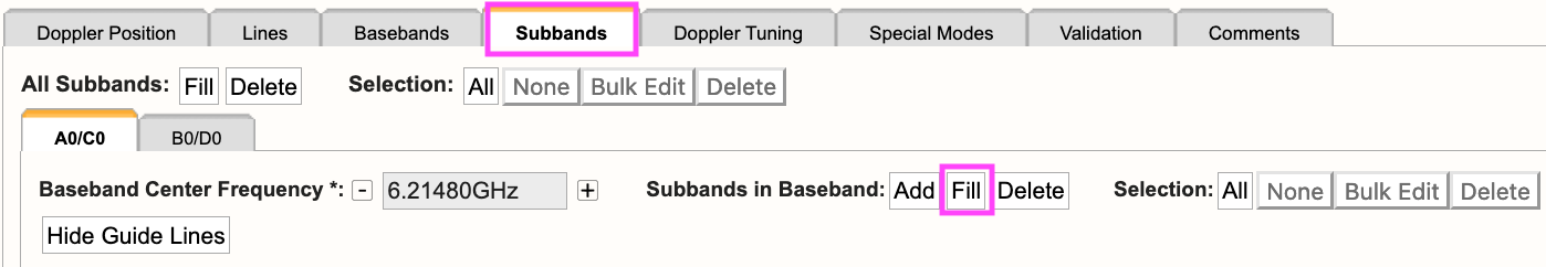 |
|
Figure 3.3.3c: Adding continuum subbands in the Subbands tab using Fill. |
After selecting Fill, the user will be presented with a pop-up box containing the following parameters:
| Bandwidth |
This defines the bandwidth of each continuum subband. |
| Number of Subbands |
The maximum number of subbands per baseband will vary depending on the sampler mode (3-bit or 8-bit) and how many baseline board pairs have been used so far by the generated spectral lines. |
| BlBPs |
Number of baseline board pairs to stack per subband. |
| Polarization |
Full (RR, LL, RL, and LR), Dual (RR and LL), or single (RR or LL) |
| Array Summing |
None should be used for spectral line resources. |
| Recirculation |
This can be utilized per subband to increase the resolution without increasing the number of BlBPs, i.e., correlator resources. |
| Place first subband in Grid |
The default is to start at the #2 subband. You may change this to start at a different subband, e.g., #1. |
Doppler Tuning Tab
You are required to enable the Doppler tuning for at least one baseband doing so will also enable a Doppler Report located below the Doppler tuning settings (see Figure 3.3.3d).
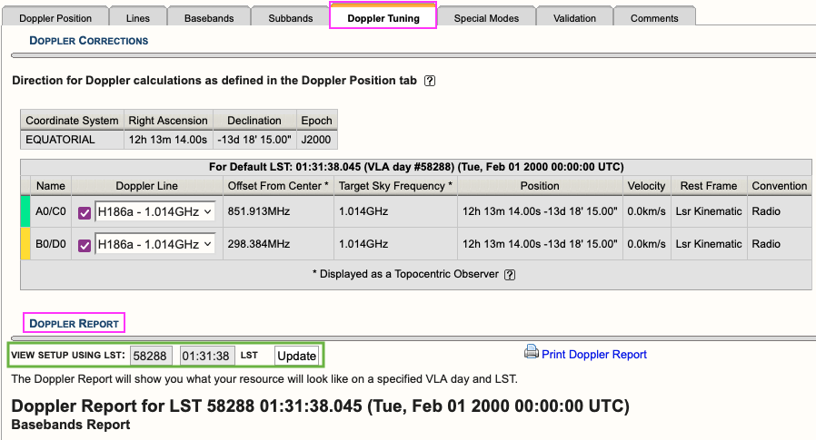 |
|
Figure 3.3.3d: Doppler Tuning tab showing an example of a Doppler Report. |
You may update the report to view the setup for a given VLA LST day and time. This will recalculate the values in the baseband tables below and will allow you to see what the on-the-sky values ("Script Computed Center Frequency" column) will be on the set day and time. The default values are 58288 01:31:38 LST which translates to 2000Feb01 00:00:00 UT.
Special Modes Tab
RFI blanking can be enabled for the entire resource. For more details, refer to the RFI Blanking section.
Validation Tab
If the resource does not validate and it's not clear why, contact the NRAO Science Helpdesk via the RCT. Contacting us via the RCT will append a log file to the ticket so we can take a deeper dive into the resource errors.
Comments Tab
You may provide comments as notes to yourself for future reference.
Custom Type Frequency Sweep Setup
On November 8, 2023, a new Resource Catalog Tool was introduced which changes the way custom resources are created. This section will cover the creation of a custom Frequency Sweep resource. If you have questions or issues, please contact us through the NRAO Science Helpdesk.
Create a Frequency Sweep Resource
After selecting to create a new instrument configuration, the New Resource Wizard pop-up box will appear with several options.
To create a frequency sweep resource select,
- Frequency Sweep
- Array Configuration: This will set the recommended default correlator integration time, which can be changed later if needed.
- Observing Band: Be sure to select the correct observing band since it cannot be changed at a later step.
- Sampler Input Mode: 8-bit or 3-bit, mixed mode can be chosen in the Basebands tab
- Name: This should match the name of the resource entered in the PST.
- Finally, select the Generate button.
Basics Table
Near the top you will find the Basics info table (see Figure 3.3.4a) were you can change the name of the resource and the correlator integration time.
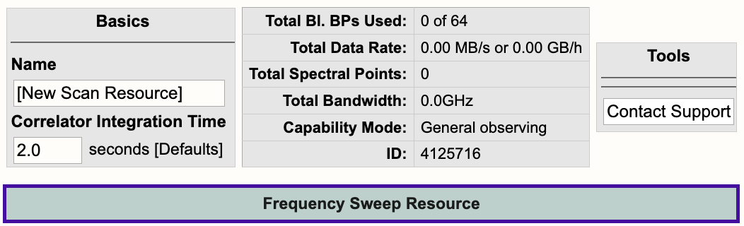 |
|
Figure 3.3.4a: Frequency Sweep Basics info table. |
Below is a description of the parameters in the Basics table.
| Name |
Be sure to use unique names for all different resource setups and do not use special characters. |
| Correlator Integration Time (seconds) |
The correlator integration time would have been set when the resource was initially created by selecting one of the array configurations. This can be modified in the table if you do not wish to use a default setting. For more details, refer to the Time Resolution and Data Rates section of the Observational Status Summary (OSS). |
| Total Bl.BPs Used |
This indicates the total baseline board pairs (BlBPs) used, i.e., correlator resources. The starting number will always be zero and will increase as lines and continuum subbands are added and when more baseline board pairs are used per line. |
| Total Data Rate |
The data rate of the resource will increase as lines and continuum subbands are added. Keep in mind the minimum and maximum data rates: Time Resolution and Data Rates. |
| Total Spectral Points |
The total spectral points will increase as the number of requested BlBPs increases. For a more detailed explanation, refer to the Recirculation vs Baseline Board Pairs section. |
| Total Bandwidth (GHz) |
This will display the sum of all subband bandwidths across all basebands in GHz. |
| Capability Mode |
The will display the capability mode of a resource, e.g., general, shared risk, or resident shared risk observing. This will depend on the total data rate and certain other settings described in the OSS. |
| ID |
This is the resource ID. |
| Contact Support |
Selecting this button will allow you to contact the NRAO Science Helpdesk. |
Lines Tab
In the Lines tab (Figure 3.3.4b), you may either enter the line information one-at-a-time by selecting Add Line or import a text file containing a list of lines by selecting:
Import Spectral Lines → Browse (select the txt file containing the lines you want to import/upload) → Upload → Done (if using Firefox)
(Note, if you are using Firefox you will be required to select the Done button after selecting Upload to complete the import. Otherwise, selecting Upload will complete the import.)
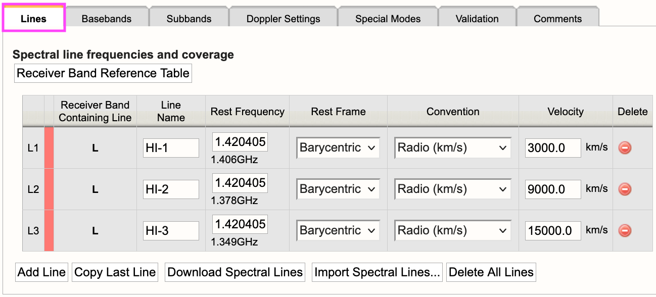 |
|
Figure 3.3.4b: Frequency Sweep Lines tab. |
For each line you will need to provide the following information:
| Line Name |
Do not use special characters and keep the name relatively short. |
| Use Line in Automated Setup (all/none) |
You may choose which lines are used in the automated setup. This means you can upload a set of lines and only use some of them or use this option as a way to partially automate/manually setup your resource. |
| Rest Frequency |
Rest frequency of the line you wish to observe in GHz. |
| Rest Frame |
LSR, Topocentric, Barycentric, Geocentric |
| Convention |
Radio (km/s), Optical (km/s), Redshift (Z), Relativistic (km/s) |
| Velocity (km/s) |
The line-of-sight velocity at which the line should be observed. |
Below is an example of a line text file for a Frequency Sweep resource. For more details, refer to the OPT manual. Note, you may also use the same syntax you would use for a spectral line text file. This means you may export a set of lines from an existing resource in the RCT-observing (this is the RCT used in conjunction with the OPT when setting up observations).
#Line name; Rest frequency; Rest frame; Velocity convention; Velocity; Minimum range; Channel separation; Polarization products
HI-1; 1.420405751GHz; Barycentric; Radio; 3000.0km/s; 100.0km/s; 1.0km/s; FULL
HI-2; 1.420405751GHz; Barycentric; Radio; 9000.0km/s; 100.0km/s; 1.0km/s; FULL
HI-3; 1.420405751GHz; Barycentric; Radio; 15000.0km/s; 100.0km/s; 1.0km/s; FULL
Basebands Tab
Set the baseband center frequencies and sampler input mode.
Subbands Tab
The lines added to the Lines tab will appear as a guide for placing continuum subbands with more correlator resources, e.g., BlBP stacking and recirculation. For more details on stacking BlBPs and increasing recirculation, please refer to the Recirculation vs Baselineboard Pairs section.
For each baseband, continuum subbands can be added one-at-a-time by selecting Add or use the recommended Fill button at the "Subbands in Basebands" level (see Figure 3.3.4c). Manually adding subbands one-at-a-time will require the user to select the Add button, then select the central frequency range of each continuum subband by choosing the desired range in the drop-down menu located in the subbands table. With either option, bulk filling the subbands or manually adding the subbands, the user can edit individual subbands as needed.
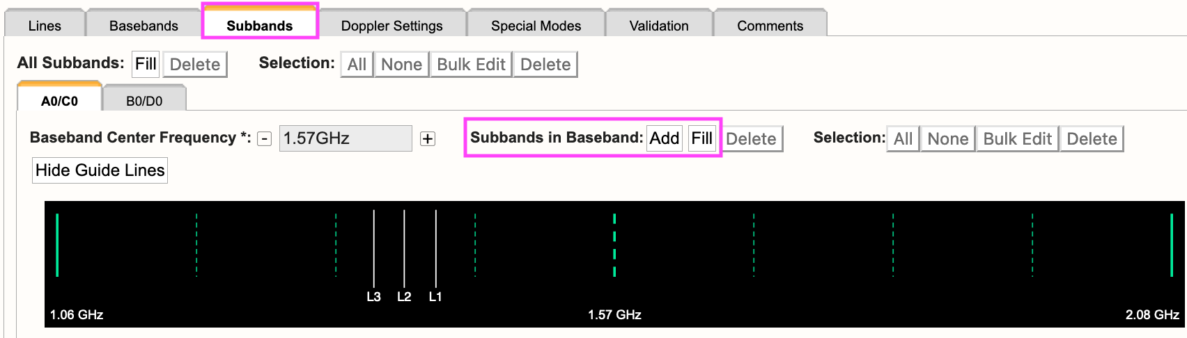 |
|
Figure 3.3.4c: Subbands tab. |
Selecting Fill, the user will be presented with a pop-up box containing the following parameters:
| Bandwidth |
This defines the bandwidth of each continuum subband. |
| Number of Subbands |
The maximum number of subbands per baseband will vary depending on the sampler mode (3-bit or 8-bit) and how many baseline board pairs have been used so far by the generated spectral lines. |
| BlBPs |
Number of baseline board pairs to stack per subband. |
| Polarization |
Full (RR, LL, RL, and LR), Dual (RR and LL), or single (RR or LL) |
| Array Summing |
None should be used for frequency sweep resources. |
| Recirculation |
This can be utilized per subband to increase the resolution without increasing the number of BlBPs, i.e., correlator resources. |
| Place first subband in Grid |
The default is to start at the #2 subband. You may change this to start at a different subband, e.g., #1. |
Doppler Settings Tab
This is optional. For more details, refer to the Doppler Tuning Tab portion of the Spectral Line Setup section.
Special Modes Tab
RFI blanking can be enabled for the entire resource. For more details, refer to the RFI Blanking section.
Validation Tab
If the resource does not validate and it's not clear why, contact the NRAO Science Helpdesk via the RCT. Contacting us via the RCT will append a log file to the ticket so we can take a deeper dive into the resource errors.
Comments Tab
You may provide comments as notes to yourself for future reference.
Custom Type Continuum Setup
On November 8, 2023, a new Resource Catalog Tool was introduced which changes the way custom resources are created. This section will cover the creation of a custom continuum resource. If you have questions or issues, please contact us through the NRAO Science Helpdesk.
Generate a Continuum Resource
If you prefer not to use an NRAO Default resource, for example for On-The-Fly Mapping observations, you may create a custom continuum resource in your personal catalog. These steps are applicable to wide band continuum resources for 8-bit and 3-bit instrument configurations. At any time you can click on the [?] icon to bring up a window with more information on the selected topic.
First, select the personal catalog/group you wish to create the resource in, then do the following to create an 8-bit or 3-bit resource.
FILE → CREATE NEW → INSTRUMENT CONFIGURATION
You will then be presented with the New Resource Wizard (Figure 3.3.5a). Here you can select the type of resource (see the other sections on spectral line, frequency sweep, or manual setups), the array configuration, and give the resource a name.
 |
|---|
| Figure 3.3.5a: New Resource Wizard. |
Once you select Continuum, the Wizard will expand as indicated in Figure 3.3.5b below to give you more options. If you click on the Generate button before the Continuum options become available then this session of the OPT will crash. If that happens, please contact the NRAO Science Helpdesk so that this session can be terminated.
 |
|---|
| Figure 3.3.5b: Expanded Wizard for Continuum setup |
Here you will select the array configuration for the resource - this will adjust the Correlator Integration Time according to the NRAO default for that observing band. You can enter your desired value later. The Sampler Input Mode has two options: Two 1-GHz 8-bit samplers (A0/C0 and B0/D0) or Four 2-GHz 3-bit samplers (A1/C1, A2/C2, B1/D1, and B2/D2). Also specify a descriptive and useful name the resource. When all this has been done, click on the Generate button to create your new Continuum resource.
Important Note: After typing in any of the text fields, click somewhere else on the page (not in another field) to allow the entry to be applied (and saved to the data base) and always be patient when updating fields or navigating to different tabs.
A new 3-bit K-band continuum resource has been generated (Figure 3.3.5c).
 |
|---|
| Figure 3.3.5c: K-band resource created by Wizard. |
Now that you have generated an 8-bit or 3-bit resource, we will walk you through the general layout of the tabs. With this knowledge, you will also be able to create a wide band continuum or frequency sweep resource. To create a spectral line resource, refer to the Spectral Line Resources section for a more detailed guide.
For 8-bit, 3-bit, and 3/8-bit mixed-mode instrument configurations you will see a graphical visual of the basebands at the top of the screen and under the Subbands tab. In addition, there is an information box located at the top right indicating the total Bl. BPs used, total data rate, total spectral points, total bandwidth, and capability mode, i.e., General Observing or Shared Risk. Figure 3.3.5c (above) is an example of the information you will be presented at the start of creating an 8-bit resource. Note, all completed actions made while working on a resource are automatically saved.
Basics Table
Near the top you will find the Basics info table (Figure 3.3.5d) where you can change the name of the resource and the correlator integration time.
|
Figure 3.3.5d: Continuum Basics info table. |
Below is a description of the parameters in the Basics table.
| Name |
This should be distinctive from other resources and match the name of the corresponding resource used in the proposal. Do not use special characters and it is probably best to keep the name relatively short. |
| Correlator Integration Time (seconds) |
The correlator integration time would have been set when the resource was initially created by selecting one of the array configurations. This can be modified in the table if you do not wish to use a default setting or if the default is no longer correct once the observing band has been determined. For more details, refer to the Time Resolution and Data Rates section of the Observational Status Summary (OSS). |
| Total Bl.BPs Used |
This indicates the total baseline board pairs (BlBPs) used, which is a measure of the required correlator resources. The starting number will always be zero and will increase as lines and continuum subbands are added and when additional baseline board pairs are stacked on a line. The maximum number of available baseline board pairs is 64. |
| Total Data Rate |
The data rate of the resource will increase with shorter correlator integration times and as lines and continuum subbands are added. Keep in mind the minimum and maximum data rates listed at Time Resolution and Data Rates. |
| Total Spectral Points |
The total number of spectral points will increase as the number of requested BlBPs increases. The number of spectral points in a subband is the product of number of channels, number of polarizations and number of baseline board pairs. The total here is the sum over all subbands. For a more detailed explanation, refer to the Recirculation vs Baseline Board Pairs section of the OPT manual or the Spectral Line Resources section. |
| Total Bandwidth (GHz) |
This will display the sum of all subband bandwidths across all basebands in GHz. This sum has no correction for overlapping subbands but note that overlapping subbands do not physically add to increasing continuum sensitivity. |
| Capability Mode |
This will display the capability mode of a resource, e.g., general, shared risk, or resident shared risk observing. This will depend on the total data rate and certain other settings described in the OSS. |
| ID |
This is the unique resource identification number. |
| Contact Support |
Selecting this button will allow you to contact the NRAO Science Helpdesk while silently supplying data specific to this resource to the ticket. |
Below is the description of each tab element / page in the resource.
 |
| Figure 3.3.5e Baseband Tab (click to enlarge) |
| Tab | Description |
|---|---|
| Basebands |
|
 |
| Figure 3.3.5f Subbands Tab (click to enlarge) |
| Tab | Description |
|---|---|
| Subbands |
|
 |
| Figure 3.3.5g Special Modes Tab (click to enlarge) |
| Tab | Description |
|---|---|
| Special Modes |
|
 |
| Figure 3.3.5h Validation Tab (click to enlarge) |
| Tab | Description |
|---|---|
| Validation |
This tab shows a summary of the instrument configuration you have created, a table of the Subband Grid Boundaries, and a table of the BlBPs in the correlator quadrants. If there is a problem with the resource, a warning or error message will appear in the interface feedback strip at the bottom. |
 |
| Figure 3.3.5i Comments Tab (click to enlarge) |
| Tab | Description |
|---|---|
| Comments |
This tab shows an entry field where you can add comments to your resource. Note that this comment field does not override the automatically generated comment for spectral line where the rest frequency of line is given. |
Always double check your proposal to make sure your custom resource follows what you proposed to do.
If there is a need to modify the existing resource, after generating a resource and attaching it to scans in an SB in the OPT, rename or copy it to a new name and make the modifications in the resource with the new name. This adjusted resource has to be re-attached to the scans in the SB, replacing the faulty resource. The easiest way to do this is with the Bulk Edit Scans tab on the selected SB. Having a different name for the two resources is extremely useful in checking whether the edit was successful and whether scans with the old resource have been overlooked.
Legacy/Manual Spectral Line Setup
Creating a spectral line resource is similar to creating wide band resources as outlined in the previous section, except for the more advanced specification of the subbands and subband frequency tuning and possible Doppler setting of the frequencies. Eventually, resources with the requested correlator settings will be pre-filled from information submitted to the PST during the observing time allocation procedure. However, at this stage none of this has been implemented.
For how and when to use this observing mode, refer to the Spectral Line section of the VLA Observing Guide.
The NRAO Defaults resource catalog contains full polarization dual IF pair spectra-polarimetry resources (the wide band continuum resources). If they appeal to you, you can copy/paste them in a personal catalog just as for the wide band resources above and edit them as needed. Check the spectral line resource properties very carefully as the spectral line resources in the NRAO Defaults have a fixed sky frequency whereas you probably want to use a rest frequency in combination with Doppler setting. Most likely, however, you will opt to create your own resource, just like creating a wide band resource previously. Some items that need extra attention are described below, but first a small detour to outline the options for creating large numbers of narrow frequency channels.
Setting Up Spectral Line Resources
After generating a new resource within your project's catalog (or personal catalog), we will now guide you through the tabs of an 8/3-bit resource on how to setup a spectral line resource. For a more detailed guided tour of a spectral line setup, with screen captures, refer to the Multi-band, Multi-spectral Line, and Continuum Tutorial.
| Tab | Description |
|---|---|
| Basics |
Name the resource, select a receiver band, enter the correlator integration time (refer to the OSS for the appropriate integration time per configuration), and add any comments for your personal use. |
| Lines |
Specify the sky position for which your observations should be Doppler set; you can use the Import Source Position button to use a predefined source from one of your source catalogs in the SCT. If you have more than one source, you can specify an average velocity, a separate line for each source velocity or create a new resource per source. Do not specify a position if you are specifying an exact sky frequency for your lines.
|
| Basebands |
For the high frequency bands (K, Ka, and Q) the default is to use 3-bit samplers covering 8 GHz bandwidth using four 2 GHz basebands, but you may select the 8-bit system to use two 1 GHz basebands. For all other bands the default is to use the 8-bit setup. If 3-bit selection is not possible, copy (and edit) a resource from the NRAO Defaults catalog. For 8-bit resources, ignore the message that there are no subbands defined.
|
| Line Placement |
The lines you specified earlier will appear in a summary table. For each of the lines you want to observe click on the Generate button, which will pop-up a dialog window for confirmation. This will generate a subband with a subband bandwidth which covers at least the velocity range requested, with enough baseline board pairs assigned (within the recirculation factor allowed). It aims to cover the bandwidth with spectral channels that are at least as narrow as the requested separation with the specified polarization characteristics. When created, the part of the baseband around the line will be shaded lighter to show the allocation in the baseband (though it may be too narrow to be distinguished). If a line can be observed with more than one baseband, there is the option to select the baseband. If you hit the Generate button more than once you will generate identical subbands without actually increasing the sensitivity for that line. |
| Subbands |
Every baseband tab will now show a table with the subbands that were generated during the Line Placement step which covers each individual line. The color assigned to a subband indicates which of the four correlator quadrant's baseline board pairs are assigned to it (in continuum typically 16 subbands have the same quadrant color) and currently for 8-bit setups you may generate up to 32 subbands in either baseband. You have the freedom to modify the subband bandwidths, but note that each doubling of the bandwidth requires a doubling of the number of BlBPs or recirculation factor to retain the channel frequency width (the default behavior is to keep the number of baselineboard pairs and recirculation constant, doubling your channel separation with each doubling of the subband bandwidth). Changing the number of polarization products has a similar effect. If subband bandwidths of less than 128 MHz are used, enable Recirculation to reduce the use of the limited amount of BlBPs (see above).
|
|
(go back to) Basebands |
You may need to go back to the Basebands tab to adjust the baseband center frequencies if a line(s) is too close to a subband boundary (within 6 MHz from the subband edge). Once the baseband centers are set, typically after the subband step, select for each baseband the Doppler Line setting characteristics. That is, from the list of lines specified in the Lines tab define the line that will be used to calculate the Doppler shift of the entire baseband for the sky position entered in the Lines tab. Formally your Doppler frequency will be correct for only one line per baseband at the start of your observation, but in practice the differences between the lines in a baseband usually are small enough to correct for in post-processing. This Doppler setting "line" does not have to be observed as that line, but it needs to be specified as a line option (with velocity and definitions) in the Lines tab. For example, one can specify a pseudo-line which is the baseband center frequency, skip generating a subband for it (as it falls on a 128 MHz boundary), but select it as the Doppler setting frequency. |
| Validation |
This allows you to inspect your setup in terms of frequencies and correlator resources (i.e., baseline board pair allocations). Check your resource, from top to bottom. If you create more than one resource, check each of the resource properties using the Show/Edit icon for each catalog entry. |
 ) to the right of the row that needs to be deleted.
Always double check your proposal to make sure your custom resource follows what you proposed to do.
After all this data entering, make sure you check your catalogs for correctness. It is important that your frequencies (with Doppler definitions) are correct before creating scans in the OPT, and before storing to disk or sharing your catalogs with your collaborators.
If there is a need to modify the existing resource, after generating a resource and attaching it to scans in an SB in the OPT, rename or copy it to a new name and make the modifications in the resource with the new name. This adjusted resource has to be re-attached to the scans in the SB, replacing the faulty resource. The easiest way to do this is with the Bulk Scan Edit tab on the selected SB. Having a different name for the two resources is extremely useful in checking whether the edit was successful and whether scans with the old resource have been overlooked.
Resource Search
The Resource Catalog Tool has two search options located in the upper left (see Figure 3.4.1) which allows the user to search within existing catalogs in their local RCT area.
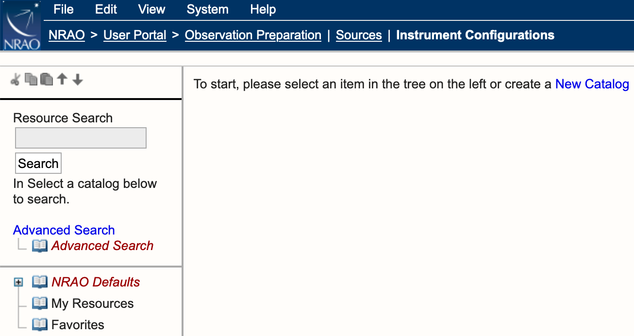 |
|
Figure 3.4.1: Resource Catalog Tool search options. |
Resource Search
The Resource Search allows the user to search for a resource or a group of resources by selecting one of the catalogs in their list below the search area and typing in the text box a resource name or a letter within the name, i.e., a wildcard search.
Example search options (see Figure 3.4.2):
- Select NRAO Defaults catalog
- Type in the letter K in the search field.
- Select Search.
- The results return all resources with the letter K in the name under the NRAO Defaults catalog.
Note, below the Advanced Search option will be numbered Search Results. The search results for both types of searches will be remembered per RCT session.
 |
|
Figure 3.4.2: Example of Resource Search results. |
Advanced Search
The Advanced Search (see Figure 3.4.3) option allows the user to narrow down the search criteria by using the search parameters and selecting visible (except for the NRAO Defaults - this will be added) and hidden catalogs as part of the search.
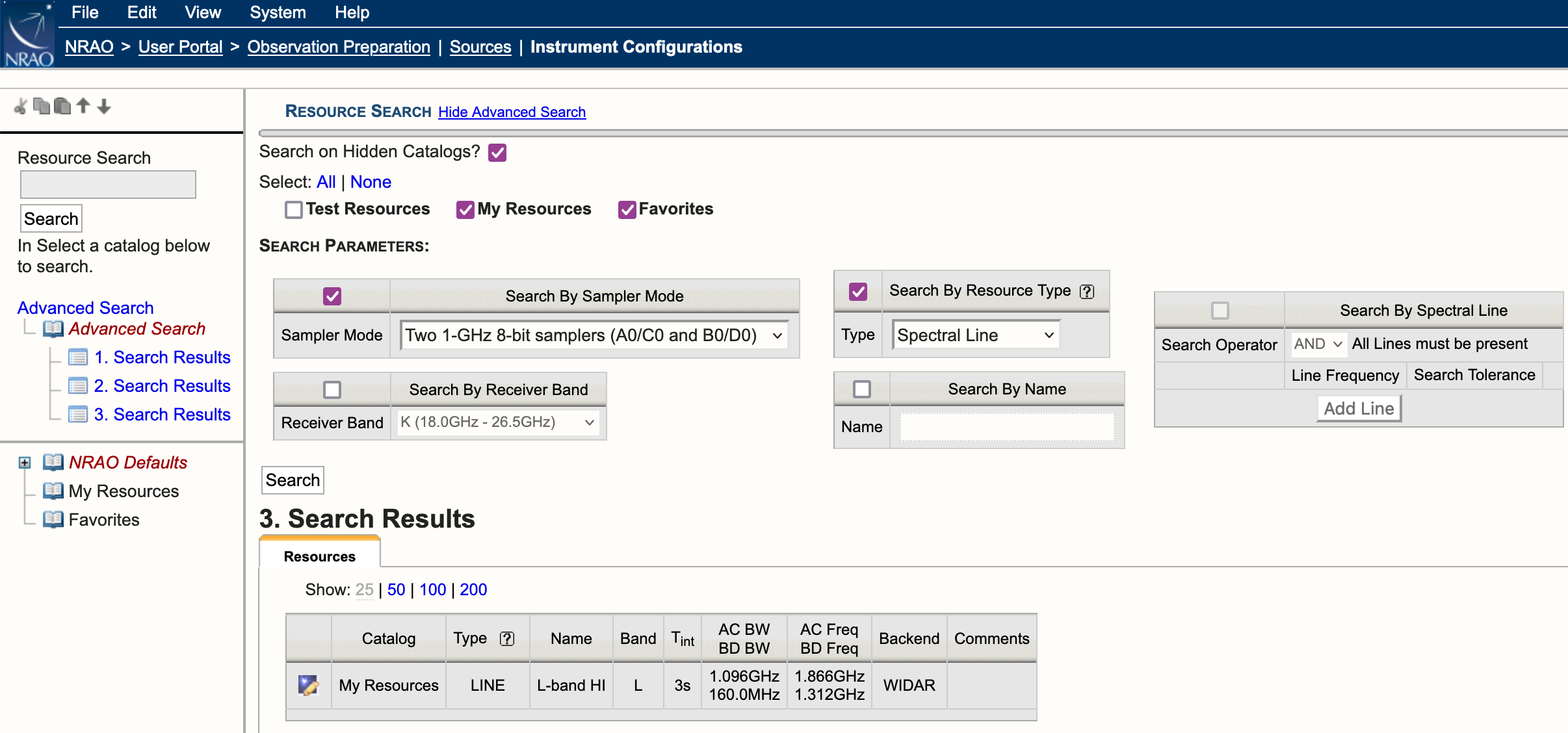 |
|
Figure 3.4.3: Advanced Search example. |
As seen in Figure 3.4.3 above, there are five search parameters which can be activated by checking the box in the upper left corner of each.
Search By Sampler Mode
- Two 1-GHz 8-bit samplers (A0/C0 and B0/D0)
- Four 2-GHz 3-bit samplers (A1/C1, B1/D1, A2/C2, and B2/D2)
- Two 2-GHz 3-bit samplers (A1/C1 and A2/C2) and a single 1-GHz 8-bit sampler (B0/D0)
- Single 1-GHz 8-bit sampler (A0/C0) and two 2-GHz 3-bit samplers (B1/D1 and B2/D2)
Search By Receiver Band
- 4 (54.0MHz - 86.0MHz)
- P (224.0MHz - 480.0MHz)
- 4/P (54.0MHz - 480.0MHz)
- L (1.0GHz - 2.0GHz)
- S (2.0GHz - 4.0GHz)
- C (4.0GHz - 8.0GHz)
- X (8.0GHz - 12.0GHz)
- Ku (12.0GHz - 18.0GHz)
- K (18.0GHz - 26.5GHz)
- Ka (26.5GHz - 40.0GHz)
- Q (40.0GHz - 50.0GHz)
Search By Resource Type
- Spectral Line
- Frequency Sweep
- Continuum
- Manual
- Legacy
Search By Name
Enter the name of a resource or a wild card.
Search By Spectral Line
This only works if Search By Resource Type is not selected (see Figure 3.4.4). Users may add one or more lines or an approximate rest frequency of a line in GHz or MHz with a search tolerance (10.0MHz is the default).
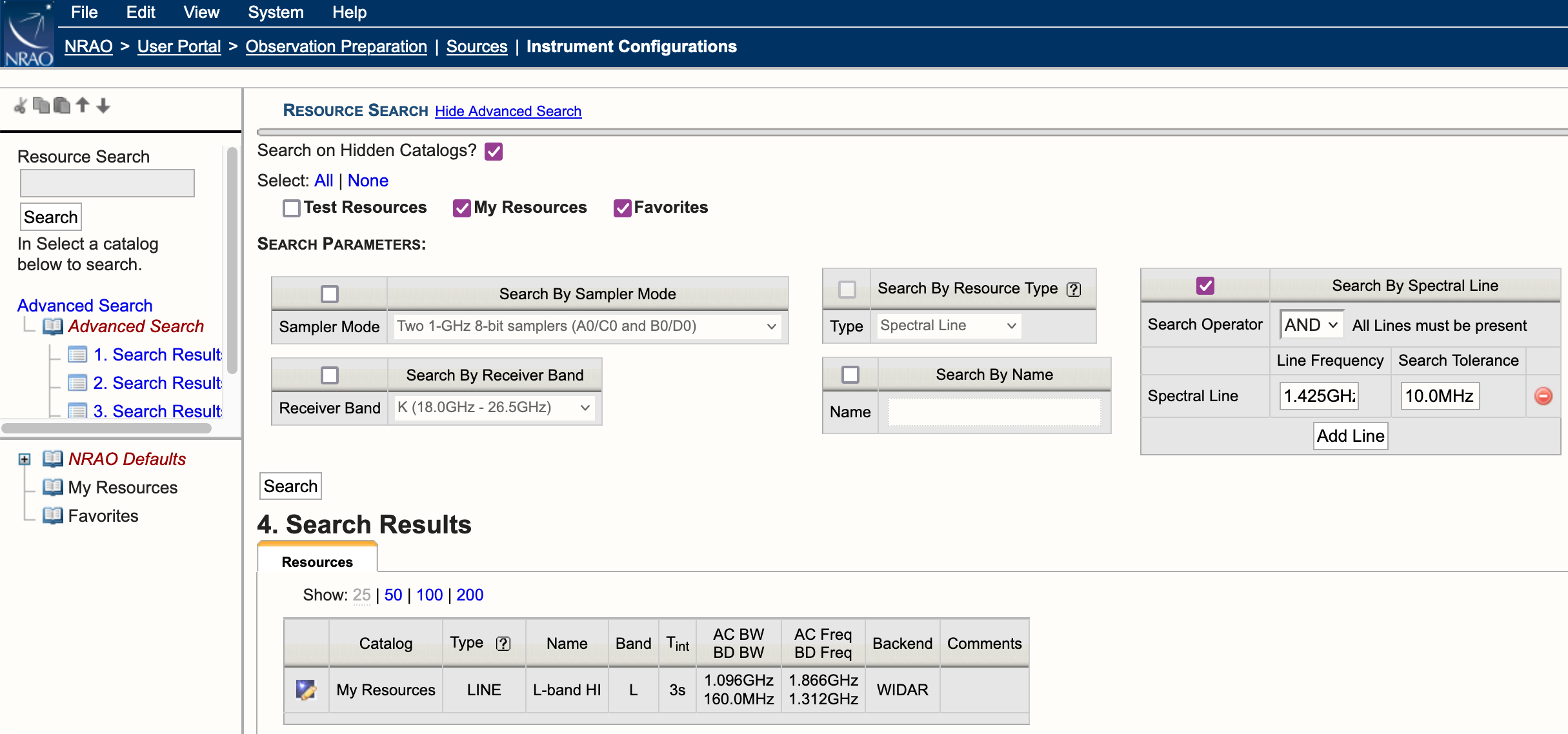 |
|
Figure 3.4.4: Example use of Search By Spectral Line. |
Channel Averaging (temporarily disabled)
Since we are unable to support channel averaging (also known as frequency averaging) at this time, it has been temporarily disabled in the RCT.
For continuum observations, the nominal correlator output with 64 full polarization, 2 MHz-wide frequency channels is more than needed to determine the delay and bandpass shape. That is, it does unnecessarily add to the total data rate and data volume and thus to the total transfer and post-processing time. Reducing the number of output channels while retaining the full bandwidth by averaging frequency channels is thus generally beneficial for wideband continuum setups.
The VLA now supports channel averaging (sometimes referred to as frequency averaging) in the correlator. Averaging of factors of two and four for specific cases (see below) is considered commissioned and available under the General Observing capabilities. Averaging of higher factors and/or for other cases may be offered under the Resident Shared Risk Observing program. The ultimate intention is to expand the use and possibly making it the default observing mode for wideband continuum. As there may be noticeable observational effects, a more detailed description to assess the suitability of frequency averaging for an observation can be found in EVLA memo 199 and the section about Chromatic Aberration in the OSS.
Channel averaging in General Observing capability mode is only offered under these conditions:
- Wideband continuum observations using 3-bit setups (frequency bands above 4 GHz, C- through Q-band)
- Frequency averaging factors are two or four (from 2 MHz to 4 MHz or 8 MHz continuum channels)
Note, OTF or Subarray observations are not allowed to use frequency averaging at this time.
The above implies that only 128 MHz full polarization subbands in all four basebands qualify for channel averaging, but this restriction may change in the future. So if the goal of a resource is to observe spectral lines in one or more basebands, where typically one would either reduce the subband bandwidth or increase the number of channels to maximize the spectral resolution, this dissatisfies the condition above.
Averaging frequency channels is implemented using the RCT. Create your own named resource, e.g., by copying one of the default NRAO 3-bit resources to your own catalog and rename it to reflect the change.
To edit all subbands across all basebands, take the following steps in the Subbands tab of your resource (Figure 3.5.1):
- Click on the All button in the All Subbands section,
- Select the Bulk Edit button,
- Select the averaging requested using the bulk edit menu (Figure 3.5.1). Once you have selected the desired channel averaging, click the Apply button.
|
|
|---|
| Figure 3.5.1: Bulk scan edit subbands option for selecting frequency averaging. |
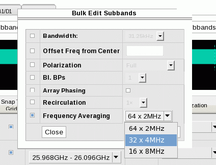
Alternatively, to edit only the subbands within a selected baseband, take the following steps in the Subbands tab of your resource (Figure 3.5.2):
- Select the baseband, e.g., A1/C1,
- Click on the All button in the Subbands in Baseband section,
- Select the Bulk Edit button,
- Select the averaging requested using the bulk edit menu and select the appropriate value in the pull-down menu for channels. Once you have selected the desired channel averaging, click the Apply button.
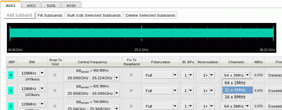 |
|---|
| Figure 3.5.2: Select frequency averaging per subband. |
Additional Resource Features and Restrictions
Although the VLA data transmission and correlation is very flexible, there are some restrictions. An overall restriction is that there are only a total of 64 baseline board pairs available. The transmission restrictions, most notable in the higher frequency bands (K, Ka, and Q) are noted further below. The correlator restrictions and a possible remedy are described here first.
32 Subbands per 8-bit Baseband - Data Path One
The nominal data path through the correlator is configured to yield up to 16 subbands per sampling baseband; this nominal data path is internally referred to as “DP0”. There are four 3-bit sampler basebands (in pairs of two spanning up to 5 GHz, a 3-bit transmission restriction) and two 8-bit sampler basebands. For plain continuum, these basebands will be (typically) assigned 16 or 8 “continuum subbands” of 128 MHz to cover the entire baseband frequency range (except for observations below 2 GHz). If one defines subbands for spectral line work, either by using the automated setup or setting them up manually, the distribution of the line subbands will determine the allowed number of subbands available for continuum in each baseband. We recommend defining the line subbands before defining the continuum subbands if line observations are the goal.
Continuum or frequency-sweep observations in 3-bit or 8-bit will generally not have any issues with the number of basebands in DP0 although other restrictions like the maximum number of baseline board pairs and maximum data rate still apply.
Spectral Line Work in 3-bit
A baseband with N assigned line subbands will have room for (16-N) continuum subbands. That is, in 3-bit setups the maximum number of subbands per baseband is always 16 and the stream will always use the nominal data path (i.e., DP0); unused subbands in a (or an unused) baseband cannot be reassigned to function as extra subbands in other basebands. The “Fill option” in the subbands tab in the RCT should only define up to (16-N) 128 MHz subbands (using a baseline board pair each) as determined for each of the four basebands, keeping in mind the total maximum of 64 baseline board pairs for the entire (line+continuum) setup. If the distribution of the continuum subbands over the basebands is not as desired, and all 16 subbands in a baseband have been assigned, it may be possible to move particular line subbands from one baseband to another and moving the continuum subbands in the opposite direction.
Spectral Line Work in 8-bit
Identical to the 3-bit case, the nominal data path, DP0, allows for 16 subbands in an 8-bit sampled baseband, whether used for line or continuum. As the full baseband frequency coverage can be met with eight subbands already, there will be no restrictions for up to eight line subbands defined per baseband and the Fill option in the RCT will insert additional subbands in each of the two 8-bit basebands as listed below. Note that there are different ways to invoke the Fill option with details on possible corrective actions below.
When more than eight subbands in a baseband are defined for spectral line work and it is not possible or desired to distribute the line subbands over both basebands to end up with eight or fewer line subbands in each of the basebands, adding the full baseband frequency coverage with eight continuum subbands to yield more than 16 subbands in an 8-bit baseband is possible but a little more tricky. The addition of subbands over the nominal 16 subbands in a baseband is possible because there are only two, not four, basebands in use and the extra hardware to double the number of subbands for 3-bit observing are not utilized. The 16 subbands allocated to each of the two unused basebands otherwise used in a 3-bit setup can now be reassigned to each of the 8-bit basebands using an alternative data path, internally referred to as “DP1” (data path one). Note that 3-bit cannot use this DP1 as the hardware necessary is already being used. Triggering the additional hardware reassignment to the 8-bit setup then allows for up to 32 subbands per baseband, i.e., leaving up to (32-8=) 24 subbands per baseband that can be configured for line observations while retaining the full 8-bit continuum frequency coverage. Of course, more than 24 subbands can be configured for line observations by sacrificing some of the intended continuum subbands in that baseband.
Adding subbands using the “Fill option” in the RCT and warnings about “DP1”
As mentioned before, it is highly advisable to specify the line setup before adding continuum subbands. It is also important to know that “DP0” should always be invoked for every baseband; a baseband configured to only invoke subbands in “DP1” will not yield data and actually stop observing. Therefore the following precautions should be taken when using the Fill option after finalizing the line portion of a resource - this assumes to be in the Subbands tab of the resource with the Figures 3.6.1 and 3.6.2 below for reference:
- Selecting the “Fill” next to “Subbands in all Basebands” on the left above the individual baseband tabs
- By selecting the Fill option for all basebands simultaneously, a total of (8-N) 128 MHz full polarization subbands will be added to each of the two basebands (N can be different for each baseband) to yield a total of eight (line+continuum) subbands. To obtain the maximum continuum coverage, an additional N continuum subbands should be added manually for each baseband (using the buttons at the top or bottom of the table) - check both baseband tabs. Note that the continuum subbands in the basebands, the subband pair identifier (SBP) at the left hand side of the table (e.g., Fig 3.6.1) will have a different color than the color of the baseband in the top graphic and start with number 16 indicating that these subbands are using DP1.
- In the case that there are no subband pair identifiers (SBP) with numbers below 16 (or in the color of the subband in the graphic at the top, e.g., Fig 3.6.2), for example by having no line subbands placed in the baseband by the automated setup or by having deleted all line subbands using DP0, click the colored square of one of the subbands to change its color to the default (as in the top graphic, e.g., Fig. 3.22a) and the number to zero (i.e., below 16) to invoke DP0. There is no need to do this for all possible subbands; once is enough.
- Selecting the “Fill” next to “Subbands in this Baseband” on the right of the baseband frequency in the individual baseband tabs
- By selecting the Fill option for each specific baseband, up to 32-N subbands can be added with more specific parameters (bandwidth, polarization, etc). If no line subbands are defined in the baseband, it will fill using DP0 until 16 are used up, then it will assign subbands to DP1. Otherwise, with predefined line subbands, the first 16 additional subbands will use DP1, the remainder will be configured using DP0. Either way, it is likely that there will be a subband defined using DP0 (unless they are deleted manually) and it should only be checked for having at least one subband in DP0 - a SBP number below 16 and in the color of the baseband in the graphic on top - per baseband.
- Selecting "Add Subband To Baseband" at the bottom of the table of subbands in an individual baseband tab
- Not using “Fill” but manually adding a subband to a baseband at a time will start using DP0 until 16 subbands are defined and continue to use DP1 for additionally added subbands. Again, make sure to check that at least one subband is using DP0.
 |
|---|
|
Figure 3.6.1: Correct use of data path 0 and 1 in a single baseband. Note, the change in color indicates which subband uses the additional hardware (in 8-bit). |
|
|
|
Figure 3.6.2: Incorrect use of data path 1 in a single baseband. At least one SBP should be toggled to enable data path 0 (in 8-bit). |

Ka-band Transmission Restrictions
There is an issue with specifying the frequency of IF pair AC at Ka-band. That is, tuning any part of the AC IF pair band below 32.24 GHz will not result in valid data, regardless whether this is A0/C0 or any of A1/C1 or A2/C2. Only the BD IF pair can be tuned to frequencies below 32.24 GHz; use the BD IF pair instead of AC IF pair when you only need one IF pair for your resource with a frequency tuning below 32.24 GHz. If the RCT validation detects that any part of the bandwidth of IF pair AC is tuned below this 32.24 GHz it will try to swap the AC IF pair with the BD IF pair. If this is not possible, it will issue an error (in red font) in the interface feedback strip if this frequency is specified as a fixed sky frequency. It will issue a warning (blue font) for rest frequencies, as the particular tuning depends on the details of observing date, telescope pointing direction and source velocity definitions. Note that a rest frequency above 32.24 GHz may shift to below 32.24 GHz once it is assigned to a scan in the OPT. This should give you an error in the OPT; you should be aware of this possibility and pay attention to this. However, it is better to assign IF pair BD to the resource if you anticipate this might happen, if you still have this freedom in your resource of course.
When observing very close to 32 GHz with both IF pairs, some combinations where frequency coverage of AC and BD are overlapping are not possible. Consult the NRAO Science Helpdesk for options, preferably before submitting the proposal.
The very wide bandwidth of the Ka-band receiver, from 26.5 to 40 GHz, would suggest that IF pair separations of up to ~13 GHz are possible. Restrictions in the signal path, however, limit this separation to 10 GHz (or any part of the basebands to within 12 GHz). The RCT validation will issue an error if the separation between IF pair centers of AC and BD is more than 10.5 GHz in sky frequency (with IF pair AC tuned to have the higher frequency centers). A separation of more than 10.5 GHz in rest frequency will result in a warning as, e.g., highly red-shifted lines may end up with less separation when the actual sky frequencies are calculated.
K and Q-band Transmission Restrictions
If you choose the RF signals in the different IF paths to be separated by a large amount, it is possible that the RCT will only let you create a resource where the baseband frequency center(s) in IF pair AC is higher than the baseband frequency center(s) in IF pair BD, similar to the Ka-band restriction above.
RFI Blanking
The WIDAR Station Boards provide a capability to excise or "blank" impulsive radio frequency interference on microsecond timescales, thus avoiding the corruption of the longer visibility integrations that are typically accumulated over a few seconds. This mode is particularly effective at identifying and blanking interference from radar transponders in L, S, and X Bands, especially those used for aeronautical navigation between 1.0 and 1.2 GHz. The blanking applies to the voltage sample time-series recorded for each subband on a per station (i.e., antenna) basis before cross-correlation. The voltage samples are recorded at 256 megasamples per second (~4 ns) and sample values that exceed a dynamically set threshold are flagged as bad data for a fixed dwell time and ignored. Thus by blanking in time, the whole subband is effectively blanked in frequency. Optimal values identified for the RFI Blanking mode are plus or minus 5 standard deviations in voltage and a dwell time of 10 microseconds. Typical fractions of blanked data are approximately 0.1% of data per integration per subband.
The RFI Blanking mode is currently enabled in the NRAO default continuum resources for L, S, C, X, and Ku-bands in the "NRAO Defaults" resource catalogue. Continuum resources with the feature disabled are also available in the "Alternatives" catalogue under "NRAO Defaults." The mode is disabled by default for user-generated resources, but may be enabled using a radio button toggle under the "Special Modes" tab (see Figure 3.7.1). For user-generated resources, the default state is "No" to disable blanking for all sub-bands. Selecting "Yes" enables the feature for all subbands which applies a threshold of 5-sigma and a duration/dwell time of 10 microseconds. When enabled, the blanking parameters will appear on the "Validation" tab under the columns "RFI Det. Level" and "RFI Blank. Dur." (see Figure 3.7.2). When disabled, these columns are hidden. To configure these parameters on a per-subband basis, please contact the NRAO science support staff through the NRAO Science helpdesk.
For details on the effects of RFI blanking on L-band observations, refer to the document The Impact of real-time RFI Blanking on HI 21 cm Observations.
| Figure 3.7.1: The RFI Blanking feature may be enabled or disabled under the "Special Modes" tab. |
| Figure 3.7.2: When the RFI Blanking feature is enabled, the blanking parameter values appear as new columns in the "Validation" tab. |


Observation Preparation Tool
Introduction
To access the Observation Preparation Tool (OPT), login directly to the OPT Suite URL: https://obs.vla.nrao.edu/opt. Note, to exit the tool properly, use the Exit link in the upper right corner or log out with FILE → EXIT; do not close the browser window/tab.
By the time you have reached this section of the OPT manual, you should have a populated source catalog (either personal or project related generated for you by NRAO staff) and a resource catalog populated with a custom resource create by you (or a colleague) and/or perhaps a copy of an NRAO default resource. In order to create a scheduling block (SB), you must first know the sources (science target(s) and calibrators) and resource(s) you wish to use in your observation in order to define the scans within the SB. It is useful to outline the project in terms of the program block (PB) and SBs in advance. Use information from the proposal, etc. (refer to General Guidelines) and create (re)source catalogs with only the subset of (re)sources that will be used in the SB you are about to create. Having your (re)sources in small personal catalogs is convenient and faster than having large catalogs or switching back and forth between your personal catalog(s) and, e.g., the VLA catalog. Check the remaining (re)sources for correctness before you continue.
The purpose of the OPT is to combine a source from one of your source catalogs with a resource from one of your resource catalogs, and to specify an observing mode, a time interval, and an intent for this combination. Repetitive combinations will build an observing schedule that defines an SB which may be executed by VLA operations. The sequence of scans in an SB will appear in the left-hand side column in the project tree and in the Schedule Summary on the Reports tab.
The most important rule when working in the OPT: be patient. When you click on something or enter information into a field it may take a few seconds to connect back and forth between your browser and the NRAO database. Please avoid clicking or entering before the previous action was completed. Be patient and watch the busy icon of your browser to stop (and sometimes even a bit longer).
If you have any questions, you may either submit your questions through the NRAO Science Helpdesk, request help directly from the OPT by selecting HELP → CONTACT SUPPORT, or if you have already created a scheduling block (SB) you may request help from the Validation and Submission tab. Note, if you request help from the Validation and Submission tab of an SB the project code and SB ID will be included in the subject line.
Left-hand Column
On the left-hand column of the OPT, you will see an icon menu at the top. If this is your first time using the OPT there will be nothing below the icon menu or you may see an accepted project (Figure 4.1.1).
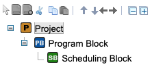 |
|---|
| Figure 4.1.1: Left-hand column of OPT. |
The OPT contains a collection of projects. Projects are subdivided in a tree of program blocks (PBs), each subdivided in scheduling blocks (SBs), which each contain scans and/or loops of scans. This column, per SB, contains the scan list, i.e., the column represents the observing schedule. In contrast to the SCT and RCT, much of the editing in the OPT will be performed in the left-hand side column as well as in the main editing window.
Icon Menu
The icon menu in the OPT has more options than in the SCT and RCT. The icons in-common have the same functionality as the icons in the SCT and RCT, but as more editing is done in the left-hand side column some extra icons (with their fly-over help tool-tip) are added. Only icons valid for the selected or highlighted items (e.g., PB or scan) are displayed. A full list of icons and their meanings is shown in the listing below. These icons do not apply to the main editing window, only to the Project tree items.
| Click to allow multiple selections for cut/copy/paste | |
| Add a new (blank) scan | |
| Add a new scan (with copy of source and hardware only) | |
| Cut (delete) selected tree item | |
| Copy selected tree item | |
| Paste selected tree item | |
| Icon menu separator (no action) | |
| Move selected item up by one in current tree level sequence | |
| Move selected item down by one in current tree level sequence | |
| Promote selected item up, above the current tree branch (out of loop) | |
| Demote selected item down, in the next current tree branch (into loop) | |
| Icon menu separator (no action) | |
| Collapse/hide all items in the selected tree | |
| Expand/show all items in the selected tree |
SB Validation Icons
New icons have been added to the OPT at the SB level indicating when an SB, scan, loop, or subarray is invalid or not validated. When the OPT validates an SB or a scan, this does not necessarily indicate that the SB is valid for observing. The VLA data analysts will still perform their validation check of all submitted SBs before approval.
| This overlay indicates the SB, scan, loop, or subarray contains invalid information. | |
| This overlay indicates the SB, scan, loop, or subarray has not been through the internal validation process of the OPT. | |
| This overlay indicates the SB, scan, loop, or subarray has a questionable setting that the internal validation is reporting. |
Note that based on the various themes the icons will appear a little different than below, which is using the Standard Light theme.
| SB Icons | Scan Icons | Loop Icons | Subarray Icons | ||||
| valid | valid | valid | valid | ||||
 |
error |  |
error |  |
error |  |
error |
| not validated | not validated | not validated | not validated | ||||
 |
warning |  |
warning |  |
warning |  |
warning |
Menu Strip
The OPT has many menu strip options. Some of the options are only accessible when editing certain items, i.e., PBs, SBs, and scans.
| File | Edit | View | Help |
|---|---|---|---|
|
Create New → Test Project → Program Block → Scheduling Block → Scan → Before → In → After → Scan Loop → Before → In → After → Subarray → Before → After |
Cut Project Copy Project Paste → Paste Before → Paste Into → Paste After To Durations Unroll Loop
|
Hide/Unhide Projects Theme
Font Size → Large → Medium → Default
|
About the OPT About Me New Features Documentation Contact Support
|
|
Refresh Project Import Project... Import Scheduling Block... Import Scans... |
|||
|
Export Project Export Scheduling Block Export Scans Export Catalogs... |
|||
|
Exit |
Project and Program Block Levels
To utilize the OPT for creating scheduling blocks (SBs), you may either use an existing approved science project under your OPT login or create a test project. To create a test project, go to FILE → CREATE NEW → TEST PROJECT. A test project will automatically generate a program block (PB) and an empty SB. For the test project, you may edit the name of the project and the PB to something more descriptive to you. As with a science project, you may add co-I's (they must have a my.nrao.edu profile) to your test project if you wish to share your observing ideas with a student, teacher, advisor, or colleague.
Project Level
Once you have created or decided on which project to work on, click on the project name in the left-hand side column. You will then be presented with the Project Details.
| Project Details | |
|---|---|
| Title |
The default is the project code (this field is editable). |
| Project Code |
Assigned proposal code at the time of proposal submission. |
| Proposal Code |
Assigned proposal code at the time of proposal submission. |
| Type |
Observing type may be simple, multiconfig, or test. |
| Telescope |
EVLA (this indicates the use of the WIDAR correlator) |
| Test Project? |
No (for science projects) or Yes (for test projects) |
| Allocated Time (hrs) |
Total approved allocated time for the project. |
| Time Used (hrs) |
Total successful time observed for the project. |
Listed below the Project Details will be the principle investigator (PI), proposal contact author, and a list of co-authors. All are listed with name and default email as indicated in their my.nrao.edu user profile. The options to receive emails (yes or no) is to allow each person on the proposal to receive email (un)submissions of SBs and the observing log for each successful observation. Note, the VLA operators do not email observing logs for failed observations. If you have a question regarding a failed observation, please contact the NRAO Science Helpdesk.
Program Block Level
To reveal the PB(s), click on the plus icon to the left of the project in the project tree. All projects will have at least one PB, some may have more depending on allocated array configurations and observing priority per observing semester and/or array configuration.
| Program Block Details | |
|---|---|
| Name |
Often written as allocated array configuration and observing priority, e.g., B (C) indicates B-configuration C-priority. |
| Scheduling Priority |
Allocated observing priority can be A, B, or C. |
| Allocated Time (hrs) |
Approved allocated time for the selected PB. |
| Used Time (hrs) |
Successful time observed for the selected PB. |
| Acceptable Configurations |
Allocated array configuration(s) for the selected PB. |
Below the Program Block Details and Acceptable Configurations is the ability to link SBs (described under Linking SBs), table of generated SB(s), and a table of execution blocks (EBs).
If you have created a test project, you may edit two of the fields: Name and Acceptable Configurations. When creating SBs under a test project, you must select a configuration. Do so by selecting the configuration (hold onto it with the mouse button) and then drag the desired configuration from the right column to the left column.
Scheduling Blocks Table
Each SB will be listed in the Scheduling Block table with 10 sort-able columns of information pertaining to the SB.
- Index (to be used when linking SBs)
- Name (when selected, will open the SB)
- Id# (each SB is given a unique identification number)
- Status (NOT_SUBMITTED, SUBMITTED, SCHEDULABLE, COMPLETED, ON HOLD, or EXPIRED)
- Executions (number of counts or repetitions for the SB)
- Total Time (total duration of all executions of an SB with N counts or N+1 counts)
- Per Execution (total duration of a single execution of the SB)
- Scheduled Start (Dynamic SBs will indicate LST start range and Fixed-date SBs will indicate LST day and time)
- Wind (selected wind (in m/s) constraints)
- Api (selected atmospheric phase interferometer (in degrees) constraints)
Execution Blocks Table
An EB is generated once an SB has been selected by the Observation Scheduling Tool (OST). If an observation is completed or failed, it will appear in the Execution Blocks table. In addition, each SB has an Executions tab. Successful and unsuccessful (i.e., failed) observations of the selected SB will also appear in the Executions tab. The Execution Blocks table contains 10 columns:
- SB ID (scheduling block identification)
- EB ID (execution block identification)
- Status (Completed or Failed)
- Duration (total length of SB)
- Started (two sets of days and times in LST and UT)
- Finished (two sets of days and times in LST and UT)
- Initial API (°) (initial atmospheric interferometry conditions)
- Initial Wind (m/s) (initial wind conditions)
- Script + VCI (If the SB was observed using the OST, the script and VCI (virtual correlator interface) files are available for download.)
Create an SB and Scans
To create an SB, first navigate to the Project and the appropriate PB. For approved science projects, it's important to select the appropriate PB. If there is more than one PB, be sure the SB(s) you will be creating contain the allocated science target(s) and resource(s) approved for the selected PB.
Create a new SB: FILE → CREATE NEW → SCHEDULING BLOCK
SB Components
After creating a new SB or selecting an existing SB you wish to edit, you are presented with six tabs in the main editing window (Figure 4.3.1). We will begin by first explaining the Information tab.
 |
|---|
|
Figure 4.3.1: Information tab example. |
Information Tab
The Information tab is used to set the scheduling constraints of the observation.
| Information Tab | |
|---|---|
| Name |
Name the SB something useful to help keep organized. |
| Count |
If count is 1, then the SB will only be observed once (successfully). If count is greater than 1, then you will have the option to add minimum days between repetitions (in LST (default) or UT) and the option, separation measured from beginning of LST range. |
| Schedule Type |
Dynamic is the default since the VLA is dynamically scheduled. This allows observers to set weather constraints so we may observe the SB in the best possible conditions for the observing band(s). This is especially important for high frequency observations. For Fixed Date allocations, the starting VLA day (i.e., modified Julian day number on the VLA schedule) and LST starting time will need to be entered. To schedule in UT time, e.g., for VLBI scheduling, you can use the UTC button. When Fixed Date is selected, many of the scheduling constraints will disappear, including the wind and atmospheric phase limit constraints. |
| LST Start Range |
The LST start range is determined by when all sources (science target(s) and calibrators) are preferably greater than 10d EL at the VLA. Multiple LST start ranges can be set per SB by clicking on the Add button. However, be careful to avoid antenna wrap issues and avoid EL limits. More information can be found in the Observing Guide. |
| Find LST Start Range (New) |
There is a new feature that can be used to find one or more LST start ranges depending on the elevation limits (see Figures 4.3.2-4.3.5). An antenna wrap may also be suggested, depending on the setup. This can be run at any time, even if an LST start range has been chosen by the user. It is suggested to rerun this if the SB length has been changed. |
|
Earliest UT Start Date/Time< and/or Latest UT Start Date/Time |
If these fields are left untouched, then the SB can be observed any time within its allocated observing semester. The earliest and latest UT start date/time can be edited to avoid observing during a certain time, such as avoiding observing too close to the Sun or if a source is interesting only during a small window of time. For example, if the earliest and latest UT start date/time are set to 2020/09/01 04:30:00 - 2020/09/04 19:45:00, then the SB can only be observed within that narrow window of time. Note: This field is editable when the SB has a schedulable status. |
|
Avoid Sunrise Avoid Sunset |
These boxes are for predictable sunrise and sunset (LST) times and not for unpredictable events such as solar flares that might happen anytime, are unpredictable, and not monitored by NRAO staff. However, selecting these boxes may be useful for low frequency observing (total electron content) as well as for high frequency observing (temperature changes in the dishes). If either of these boxes is selected it may be that your observations are not possible during the array configuration that you were allocated observing time for. Selecting the sunrise/sunset check-boxes will prevent your SB from being observed if any part of the observation would overlap with the interval between 10 minutes before and 60 minutes after sunrise/sunset. If the SB is going to be more than a couple of hours long and/or the RA is about 6 hours away from the Sun you might have to live with observing at sunrise/sunset if the observations must take place during this time of year. The alternative is to observe during a different proposal cycle. The diagram on the LST Scheduling Considerations page shows the approximate sunrise/sunset LST times as function of day of the year at the VLA. When checking the SB on the Reports tab, sunrise/sunset warnings will appear at the bottom in the interface feedback strip if there is any overlap with the chosen LST start time range and chosen date range (within the allocated configuration). If so, the SB will not run during those dates. If all the dates during the array configuration conflict with sunrise/sunset, either shorten the SB length or uncheck the box(es). It is particularly important to have possible dates near the end of the array configuration if the scheduling priority is not "A". |
| Wind and Atmospheric Phase Limit |
We recommend using the default wind and atmospheric phase limit (APL) for the highest observing band utilized in the SB. Observers may set custom wind and APL constraints. New with release 1.31 is the ability to select Atmospheric Phase Limit for self-calibration. For more information on considerations for setting the APL, please consult the weather constraints section of the VLA Guide to Observing. |
| Comments |
Observers may add notes about the SB in this field.
|
| Antenna wrap diagram |
The Observing Guide explains the antenna wrap diagram in more detail. |
 |
| Figure 4.3.2: Maximum Elevation selection, 90 deg is ok for P band (as long as there is no wrap issue) |
 |
| Figure 4.3.3: The minimum elevation also has a custom option. This is useful for D and C configurations when antenna shadowing can occur. It is advised to rerun the LST Start Range finder if either of the elevation limits have been changed. |
 |
| Figure 4.3.4: For each suggested LST start range, there is a button to select which will automatically change the LST start range for this tab and the static report tab. If there is a wrap suggested, this will need to be manually selected by the user for the first few scans. |
 |
| Figure 4.3.5: The first LST range has been selected. Note that the suggested antenna wrap will need to be manually set in the first few scans. Always double check to see if the wrap is valid. Using the Dynamic LST Validation tab can show if potential wrap issues can occur (changing a wrap partway in an SB) |
The other tabs seen in Figure 4.3.1 (Static Reports, Dynamic LST Validation, Submission, and Bulk Scan Edit), will be explained in later sections. The next step is to create a scan in the SB and understand its purpose and components.
Scan Details
To create a new scan within the SB you wish to edit, go to FILE → CREATE NEW → SCAN → IN.
The idea is to define a sequence of scans in the left-hand column, each with a source, a resource, an observing mode, a time interval, and some reason (intent). Each time a scan is added you will need to specify these items. However, it is not always straightforward to assemble the scan list in the sequence you want the first time around, and you will need to move scans around. This is easily done! That is, there is no need to panic if you make scans (a bit) out of order; it is almost straightforward to add, e.g., an extra bandpass calibration scan, to move some scans to the middle of the observation, or to redefine source loops after the main framework of your schedule is set up.
Figure 4.3.6 shows an example of a new scan using the default scan mode, Standard Observing. The "?" next to each of the parameters provide a flyover of information. The table below describes each of the Standard Observing parameters.
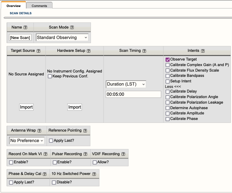 |
| Figure 4.3.6: New Standard Observing (STD) scan showing all available parameters and intents. |
|
Scan Parameters |
|
|---|---|
| Name |
Name the scan something useful to help keep organized while building the observation. Note, if you import a source before naming the scan, the scan will inherit the name of the source. You may change the name of the scan at any time. |
| Scan Mode |
Standard Observing (STD): The most commonly used mode for science targets and calibrators (e.g., complex gain (amplitude and phase), flux density scale, bandpass, delay, etc.). Interferometric Pointing (IP): Generally used in high frequency (> 15 GHz) observations to improve telescope pointing. Tipping (TIP): For measuring opacity curves. Currently not in use. Holography (H): For measuring antenna response. Internal NRAO use only. On The Fly Mosaicking (OTFM): For taking data in a constant slew that is different from compensating for Earth rotation. Solar (SOL): For a science target that is located near or on the solar disk. When a scan mode is selected, some of the scan parameters will change and the abbreviation will change in the SB scan list on the left-hand column. For a more detailed overview of the scan modes, refer to the Scan Modes in Detail section. |
| Target Source |
To select the source you wish to observe (i.e., science target or calibrator), click on the Import button, choose a Source Catalog (or Source Group within that catalog) and click on the Change button. This component pulls directly from the SCT. Any changes made to a source position within the SCT, the source must then be re-imported into the SB. New for 1.31 is the ability to filter the search across multiple source catalogs. See below in OPT 1.31 User Interface Update. |
| Hardware Setup |
To select the resource you wish to use, click on the Import button, choose a Resource Catalog (or Resource Group within that catalog) and click on the Change button. This component pulls directly from the RCT. For any changes made to a resource within the RCT, the resource must then be re-imported into the SB. New for 1.31 is the ability to filter the search across multiple resource catalogs. See below in OPT 1.31 User Interface Update. Special Notes:
|
| Scan Timing |
The scan timing determines the length of the scan. Duration(LST) is the default and the only valid option. The 5 min duration is also a default value but should be adjusted as needed. The duration of a scan includes the time it takes for the antennas to slew to the source plus the time spent on the source, i.e., slew + on source time = duration. Using the Duration(LST) scan timing mode will keep the length of the SB static. This in turn makes dynamic scheduling feasible. The OPT assumes a 20 second duration at the start of a scan to allow for receiver setup and changes in the focus and rotation of the subreflector. For observations that are switching between P-band and L-band, or P-band and S-band, more time is needed to account for the subreflector changing position. Please review the Exposure and Overhead section of the Guide to Proposing. It is possible to create SBs in On Source(LST) to investigate slew times between sources, etc., but the SB must be converted to Duration(LST) prior to submitting. This can be done best by selecting a viable LST start time in the Reports page, clicking Update to recalculate the slew times, and to make use of EDIT → TO DURATIONS from the top menu. |
| Intents |
The default is Observe Target, however it is very important to select the correct scan intent(s) for the corresponding sources. For example, the first scan for all SBs must use the Setup Intent (and no other intents). The setup intent tells the executor to set the attenuator levels on the antennas for the duration of the observation. Alternatively, the science target scans should only use the Observe Target intent and calibrators should only use their corresponding calibrator intent(s), i.e., calibrate complex gain (A and P), calibrate flux density scale, calibrate bandpass, etc.. For the calibrators, more than one scan intent may be selected. Do not use the Observe Target or Setup Intent on the calibrator scans. Note, do not use the Determine Autophase scan intent. This is only for phased VLA observations. |
| Antenna Wrap |
No Preference: The antennas will have no instructions on which direction to begin moving in AZ. CW (right): The antennas will be instructed to move clockwise in AZ. CCW (left): The antennas will be instructed to move counterclockwise in AZ. How and when to use antenna wraps is explained in the Antenna Wraps section of the Observing Guide. |
|
Reference Pointing Apply Last? |
This can only be selected on scans which are preceded by a scan using the Interferometric Pointing mode. Selecting this option on a scan will apply the pointing corrections during the observation. Note, pointing corrections cannot be applied after the observation has been taken. Therefore, it is crucial to correctly set this up in the SB. |
|
Over the Top Allow? |
This setting is still being tested and should not be selected. More details can be found under the Tipping (TIP) section. |
|
Record on Mark VI Enable? |
This setting is only used for phased VLA observations (VLBI). |
|
Pulsar Recording Enable? |
For phased-array pulsar observing only, enable this setting in order to record pulsar data for this scan. |
|
VDIF Recording Allow? |
This is only used for eLWA and radar observations. |
|
Phase & Delay Cal Apply Last? |
This setting is used for phased VLA observations (VLBI or pulsar) and should not be selected otherwise. |
|
10 Hz Switched Power Disable |
This setting disables the 10 Hz switched power calibration signal for this scan. During pulsar-mode observations the switched power should usually be disabled during pulsar scans and enabled during calibration scans. Otherwise this setting should not be used. |
| Comments tab |
You may add personal notes within the text box in the comments tab. |
Adding Scans
There are two methods for adding scans, either create a new scan or copy and paste an existing scan anywhere in the list of scans.
Add a new scan:
Select the scan you wish to add a new scan before or after.
- FILE → CREATE NEW → SCAN → BEFORE
- This will add a new scan before the scan you selected.
- FILE → CREATE NEW → SCAN → AFTER
- This will add a new scan after the scan you selected.
- FILE → CREATE NEW → SCAN → IN
- This will add a new scan in the selected SB or a selected loop. (Scan loops will be explained in the next section.)
Copy/paste a scan:
Select the scan you wish to copy.
- EDIT → COPY <name of scan>
- EDIT → PASTE BEFORE <name of scan>
- This will paste the scan before the scan you have selected or before the loop you have selected. (Scan loops will be explained in the next section.)
- EDIT → PASTE INTO <name of scan>
- This will paste the scan into a selected loop.
- EDIT → PASTE AFTER <name of scan>
- This will paste the scan after the scan you have selected or after the loop you have selected.
You may also use the copy and paste
icons located in the icon menu. The paste icon option will only paste the scan after the scan you have selected.
Scan Loops
To create a scan loop, select the scan you wish to either create the loop before or after and select,
FILE → CREATE NEW → SCAN LOOP → BEFORE (or AFTER)
Once a loop has been created, you can create new scans within the loop, copy/paste scans into the loop, and create more loops within the loop.
Scan loops are useful for creating a repetition of scans, i.e., for phase referencing (complex gain calibrator scan plus science target scan(s)). Loops can be named, be given many iterations, and contain a useful feature called Bracketed. If the Bracketed option is selected it will perform your first scan within the loop one extra time at the end of the loop.
Figure 4.3.7 shows four examples of bracketing the science target with the complex gain calibrator.
| No Loop | Normal Loop | Bracketed Loop | |
|---|---|---|---|
| individual Scans | two different orderings | should start with calibrator | |
| Figure 4.3.7: Four different bracketing styles. In these examples, Cal is an abbreviation for complex gain calibrator. | |||
Bracketing Options
- No Loop: This option does not utilize scan loops, however it is a valid option for bracketing the science target with the calibrator.
- Normal Loop: Two options are represented here.
- On the left, the calibrator is placed before the loop containing the science target and the calibrator.
- On the right, the calibrator is placed after the loop containing the science target and calibrator.
- Both options, the science target is appropriately bracketed by the calibrator.
- Bracketed Loop: The scan loop utilizing the bracket option is signified by two asterisks (**) next to the number of iterations the loop was assigned. With the bracket option selected, the first scan in the loop must be the calibrator scan so it will also be the last scan in the loop. This may not be apparent when only looking at the SB list of scans in the left-hand column, but will become more obvious when viewing the SB summary in the Reports tab.
A loop can contain any number of sources, not necessarily only a calibrator scan and a single science target scan. If your science target sources are near in the sky and you can use a single calibrator for all of the science targets, then you can group them in a loop with more than one, target scans before returning to your calibrator. Keep in mind that the total loop time should be shorter than the anticipated coherence time at our observing frequency. Loops may also contain loops. If your loop is selected, adding a new scan will place this new scan in the scan loop. The only difference with a normal scan is that this scan will be scheduled as many times as the "Loop iterations" specified, consecutively in a loop with the other sources in the loop. When finished with defining a loop, you may want to highlight it and then collapse it (using from the icon menu) for a more compact display in the tree.
Calibration
In addition to bracketing the science target(s) with its appropriate complex gain calibrator, it's important to understand when and where to add interferometric pointing (reference pointing) scans for high frequency (> 15 GHz) observations, where to place the flux density scale calibrator or bandpass calibrator (beginning, middle, or end of the SB). The Observing Guide has specific sections to help guide you on how to setup a high frequency or low frequency observation. However, the placement of some calibrators, i.e., flux density scale calibrator, will be determined by where that source is in the sky relative to the science target(s). Is it rising or setting? Double check the EL curve of the sources in the SCT (under the Images tab of a source) to help determine a good placement of the flux density scale calibrator. The placement of the flux density scale calibrator will also restrict the LST start range. There are many important factors to consider when creating an SB.
Below is a listing of specific sections within the Observing Guide helpful for setting up observations:
The Observing Guide also contains sections on Spectral Line, Polarimetry, Subarrays, Mosaicking and OTF, Moving Objects, VLBI at the VLA, and Pulsars under the Commonly Used Observing Modes section.
If at any time you are unsure of what to do or where to start with creating your SBs, please do not hesitate to contact us through the NRAO Science Helpdesk.
Filter in Import Search
Filter Source Search
Users can filter their source search in a source catalog from within the OPT. This can be useful if the source catalog in question has many source entries, such as sources used for a survey. Figure 4.3.8 shows how to activate the Filter search. Figure 4.3.9 shows the parameters available for the Filter.
Figure 4.3.9 explained:
- Source Catalog: the catalog upon which you wish to search
- Source Group: if you have groups in your catalog, you can search them individually or all of them
- Sources - Stop Filter: this will collapse the Filter options
- Name: filter by name of source
- RA: filter by RA position - Reset button resets RA to 0h 00m 0.00s (Note: when entering values you must use units)
- Dec: filter by Dec position - Reset button resets Dec to 0d 00' 0.00" (Note: when entering values you must use units
- Radius (deg): search radius in degrees based upon RA and/or Dec position - Reset button resets Radius to 1.0d
This same filter functionality is also available in the Bulk Scan Edit tab.
| Figure 4.3.8: Activating the Search Filter | Figure 4.3.9: Search filter options |
Filter Resource Search
Users can filter their resource search in a resource catalog within the OPT. This can be useful if the resource catalog in question has many resources. Figure 4.3.10 shows how to activate the Filter search. Figure 4.3.11 shows the parameters available for the Filter. Figure 4.3.12 shows what happens when you select a sampler that is not available for the receiver. Figure 4.3.13 shows that you can have multiple bands and/or samplers selected.
Figure 3.4.11 explained:
- Resource Catalog: the catalog upon which you wish to search
- Resource Group: if you have groups in your catalog, you can search them individually or all of them
- Resources - Stop Filter: this will collapse the Filter options
- Name: filter by name of source
- Filter Receiver Bands: filter by receiver band(s)
- Filter Sampler: filter by 3-bit and/or 8-bit samplers
The search results will appear as a list before the parameters section. Click on the button next to the source and select Change, or Cancel to quit.
This same filter functionality is also available in the Bulk Scan Edit tab.
| Figure 4.3.10: Activating the Search Filter | Figure 4.3.11: Search filter options |
| Figure 4.3.12: Incorrect sampler for receiver band | Figure 4.3.13: Example of multiband / sampler search results |
Check SB Setup and Duration
While creating an SB, it is important to keep in mind the allocated time in the PB you are working in. While we do allow observers to submit over the allocated time per PB, i.e., multiple SBs for multiple sources or multiple SBs to cover a wide range of LST start ranges to help improve chances of observing. The sum of the SBs or a single SB must not exceed the allocated time of a PB. For example, if a PB is allocated 4 hours, the observer may submit a 4 hour SB, a 2 hour SB with a count of 2, 2x 2 hour SBs, many SBs of varying lengths, many linked SBs (i.e., only observe one of the 2 or 3 SBs, etc.), or any combination of those options. Just be sure the sum of SBs you wish to be observed do not exceed the allocated time. For details on how to link SBs, refer to the Linking SBs section of this manual.
Static Report Tab
The Static Report tab (Figure 4.4.1) should be accessed regularly to double check the layout of the SB. This tab provides a table view of all (re)sources imported into the scans, including an instrument configuration summary, time on source summary, and a summary report of the SB. At the bottom of this tab, in the interface feedback strip, warnings and errors will appear if there are issues with the SB, i.e., antenna shadowing (if in D or C-configuration), EL limit warnings (if the EL is > 80d or < 8d (unless otherwise manually set)), if the LST start range overlaps with sunrise or sunset (if they have been selected), etc.. Below Figure 4.4.1 is a table explaining the top portion of the Static Report tab.
|
|
|---|
|
Figure 4.4.1: Example of the top portion of the Static Report tab. |
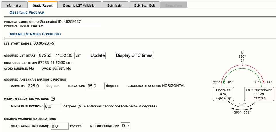
|
Static Report Tab (top portion) |
|
|---|---|
| Observing Program |
Project Code: Project (i.e., proposal) code will be displayed. If you are working on a test project you created, the project code will be your global ID with an '_n' appended (such as in Figure 4.4.1). Generated ID: Often referred to as the SB ID. Principle Investigator: PI name and email. Use your browser's Print feature to print this report, is simply a suggestion that you may use your browser's print feature to print the SB to a PDF. Before doing so, be sure to expand all loops within the SB's Schedule Summary table to capture all of the scans. |
| Assumed Starting Conditions |
Wind Constraints & API Constraints: These parameters are set on the Information tab. LST Start Range: This is set on the Information tab. Assumed LST Start: Two editable boxes are presented, the VLA day and LST start time. When checking an SB, it is important to step through the LST start range you have defined to double check time on source and EL. After entering an assume LST start, either hit enter on your keyboard or click on the Update button. Update: This button can be used to refresh (recalculate) the duration of the SB after changes have been made to scan length or to update an assumed LST start or VLA day. Display UTC times: This button can be used to change the display of LST to UTC in the Summary Report table. Computed LST Stop: After setting an assumed VLA day and assumed LST start time, the OPT will compute the VLA day and LST stop time. Avoid Sunrise & Avoid Sunset: These are set on the Information tab. Assumed Antenna Starting Direction: The default values are 225.0d AZ and 35.0d EL. These fields may be edited to see how changing the assumed antenna starting direction would affect the start of the observation. For example, if the assumed starting AZ is set to 445.0d and the first source is rising, then the antenna may need to unwrap to allow appropriate on source time. Adjusting the assumed starting AZ can also help determine if you have enough start-up time (total duration of the setup scan(s) plus the first calibrator) and which antenna wrap should be requested at the start of the SB. Coordinate System: horizontal
Minimum Elevation Warning: The default is set to the hard EL limit of the VLA antennas, 8.0d. For the safety and integrity of the EL motors, we prefer observers avoid ELs less than 10d, if their sources will allow. The OPT uses this number only as a guide when checking the LST start range of an SB and will give a warning when the EL drops below the set value during a defined assumed LST start time. Setting a minimum EL does not mean the antennas will avoid going below that EL during the observation. Observers must set an appropriate LST start range in the Information tab to avoid the required or desired minimum EL. Shadow Warning Calculations: The default is set to 0.0m (meters). Antenna shadowing only affects observations in C- and D-configuration. (Refer to the Observing Guide for more information regarding antenna shadowing.) Setting a shadowing limit (max) is only a guide for checking the LST start range of an SB. It does not mean the antennas will avoid a set shadowing limit during the observation. Observers must set an appropriate LST start range in the Information tab to avoid the desired shadowing limit. |
| Computed Summaries |
The Instrument Configuration Summary, Time On Source Summary, and Schedule Summary links will take you directly to each table or you may simply scroll down to each table. Each will be described in more detail below. Export Tables as CSV (opens in new window) will create a csv file of the Static Report tab. |
Instrument Configuration Summary
All resources imported into scans within an SB will be displayed in the Instrument Configuration Summary. This table can reveal if the correct or incorrect resources have been imported. Figure 4.4.2 is an example of the resources used in the demo SB seen in Figure 4.4.1. To reveal the subbands within the basebands, click on Show All Subbands. To minimize the view, click on Hide All Subbands or hide individual basebands. If a resource is set up to utilize the Doppler settings, it is advised to double check the OPT's calculation of the line's center frequency using Dopset. Refer to the Instrument Validation section of the Observing Guide for more details on how to verify a spectral line setup.
 |
|---|
|
Figure 4.4.2: Example of an Instrument Configuration Summary table (click image to enlarge). |
Time On Source Summary
The Time On Source Summary table (Figure 4.4.3) lists all sources used in the scans with their assigned resource, scan name, modifiers (i.e., scan intent(s)), coordinates in RA and Dec, Doppler Velocity used in the assigned resource, Doppler Line frequency of the assigned resource, min and max hour angle (HA), min and max parallactic angle (PA), and total time on source. This table is helpful in determining how much time on source a science target or calibrator with a given resource has for a specific LST start (set in the assumed LST start field in the top portion of the Static Report tab). Note, as the assumed LST start time is changed, the time on source for each source will change. This is due to the change in the antenna slew time between sources due to the change in the sources positions relative to each other on the sky.
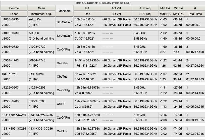 |
|---|
|
Figure 4.4.3: Example of a Time On Source Summary table. |
Summary Report
The Summary Report (Figure 4.4.4) is the most valuable for checking the overall setup of an SB. This is a table view of the scan listing created in the left-hand column. If scan loops have been utilized, be sure to click on the plus icon at the top left of the Summary Report table to expand all loops (including loops within loops). The scan mode, e.g., standard observation (STD) and interferometric pointing (IP), will be listed to the right of the scan number in the first column of this table. This matches the scan mode listing found in the tree structure in the left hand column of the OPT which has scan mode labels, e.g., STD, IP, etc. (Figure 4.4.4).
When checking an SB, it is important to step through the LST start range (defined by the observer in the Information tab) by entering different assumed LST start times at the top of the Static Report tab. This will help determine whether each observing scan (not including setup scan(s)) have the appropriate time on source (after slewing) for the entire LST start range assigned in the Information tab. The AZ and EL should also be carefully checked to avoid antenna wrap issues and EL limits. If an observing scan does not have any time on source (after slewing), that scan will be highlighted in green (as a warning). If a reference pointing (i.e., interferometric pointing (IP)) scan has less than the required 2min 30sec on source, after slewing, that scan will be highlighted in red (as an error). It is ok if setup scans do not have time on source (they will not appear in green or red). The setup scans (for setting the attenuator and requantizer gain levels) do not require the antennas to be on source.
For a more detailed check of an SB, we recommend using the built-in validation tool known as the Dynamic LST Validation tab.
OPT 1.36 User Interface Update
Under the Modifiers column, antenna wrap selection is now always visible for each scan it has been selected, e.g., requested CCW wrap (Figure 4.4.4).
 |
| Figure 4.4.4: Summary table example with requested antenna wrap included |
Dynamic LST Validation Tab
The Dynamic LST Validation (DLV) tab (Figure 4.5.1) allows observers to check their observations for a specified LST start range and several defined parameters.
Note: The NRAO staff will continue to check SBs before approving for observation. Please contact the NRAO Science Helpdesk if you encounter any issues, discrepancies, or you see a message with "unknown" severity.
New Parameters
We have added a few new parameters to help observers check their SBs:
- Antenna Wraps (CW, CCW, or no preference)
- We have made significant improvements to the DLV regarding antenna wraps. This tool will now recommend an antenna wrap direction for a given LST start range and will warn you when the incorrect antenna wrap has been selected.
- Basic tips for selecting an antenna wrap at the start of an SB:
- Select the CCW wrap, if the starting azimuth is ~70-90d.
- Select the CW wrap, if the starting azimuth is ~270-290d.
- No antenna wrap is needed if the starting azimuth and the sources following are:
- always in the north: azimuth is ~290-445d (outer wrap) or ~-85d-70d (inner wrap)
- always in the south: azimuth is ~90-270d
- Setup Scans
- Warnings will be issued if a resource (8-bit, 3-bit, or mixed-mode 3/8-bit) is missing its initial attenuator setup scan or if it’s less than the required minimum of 1 minute.
- A warning will be issued if a 3-bit or mixed-mode 3/8-bit resource is missing the 30 second requantizer setup scan(s).
- Flux/Bandpass Calibrator Scan Intent
- Warnings will be issued if a resource does not have a flux/bandpass calibrator intent selected.
- Get EL Limits From Info Tab
- This button will allow users to grab the elevation limits defined on the Information tab.
Dynamic LST Validation Parameters
As seen in the screen capture of the DLV tab (Figure 4.5.1), please note the "?" found beside each parameter. While working in the OPT, the "?" can be found throughout and contain helpful information regarding the parameters.
|
|
|
Figure 4.5.1: Dynamic LST Validator (DLV) example |

Starting Conditions
The following are editable starting conditions.
| LST Start Range | To use the same LST start range from the Information tab, select the "Get LST From Info Tab" button.
|
| LST Step |
This will allow you to step through the defined LST start range in increments of 5, 10, 15, 20, 25, or 30 minutes. The default is 5 minutes, since the LST start range can be set in 5 minute increments. |
| Assumed Antenna Starting Direction |
Azimuth This will help you determine if you have enough slew and on source time for the first calibrator scan, i.e., reference pointing, flux, bandpass, complex gain calibrator, etc.. The default starting AZ position is 225.0d.
Elevation You may also set an assumed starting elevation position. The default starting position of 35.0d is usually sufficient. |
Evaluator Settings
The following are editable evaluator settings.
| Antenna Shadowing |
Shadowing Limit (max)
|
| Elevation Limits |
Low EL Limits
High EL Limits
|
| Max Slew Time |
Time:
|
| Time On Source Minimum |
You may edit the recommended default settings for your observation. |
If you wish to reset the evaluators to the default settings, select "Reset to VLA Defaults". Note, the antenna shadowing parameters and the starting conditions will not be reset.
Running the Dynamic LST Validator
Once you are satisfied with your starting conditions and evaluator settings, select "Start Dynamic LST Validation".
The results may be grouped by evaluator, severity, LST, or all.
A "Show All" or "Hide All" results option is also available.
 |
| Figure 4.5.2: Group options for display of results |
This can be helpful when there are many messages and want to focus on a particular evaluator or severity. The messages in the table(s) may be sorted by selecting the top row of each column, i.e., by scan name, scan number, etc.. The messages within an evaluator can also be expanded (+) or condensed (-).
In addition to the editable evaluator parameters, you may see additional evaluator messages if they have been flagged in your SB. If they do not appear, then they were not used. This is likely ok. It is also ok if after you select "Start Dynamic LST Validation", you see the info message: "No Messages to display. Scheduling Block looks good."
Message Types
|
|
|
|
|
|
|
|
Evaluators
| Setup Scan |
|
| Scan Time Type |
|
| Flux Calibrator |
|
| Scan Intent |
|
| Scan Flags |
Three types of warnings may appear under this evaluator:
|
| Scan Duration - Maximum |
|
| Source Elevation - Maximum |
|
| Source Elevation - Minimum |
|
| Time On Source - Minimum |
|
| Antenna Wrap |
|
| Max Slew Time |
|
| Antenna Shadowing |
|
| Bandpass Calibrator |
|
Modify an SB and Bulk Scan Edit
After you have created an SB, you may want to make some changes (rename, re-order the scans, adjust a loop iteration, change a (re)source, etc.). Changes to an SB may be made at anytime prior to submitting. Once the SB has been submitted you will be required to cancel submission (unsubmit) to make any changes.
Copy/Paste an SB
SBs may be copy and pasted from within a PB, from another PB, or from another project you have access to. Duplicating an SB is useful if you want to re-use the basic structure of an SB, but change the (re)sources or simply change the LST start range and antenna wrap request.
Copy/Paste Procedure:
- Navigate to the PB which contains the SB you wish to copy.
- Select the SB to be copied.
- EDIT → COPY <SB name>
- Either stay in the PB to paste the SB or navigate to a different PB to then paste the SB.
- EDIT → PASTE
- The SB will then be pasted to the end of the list of SBs.
By using the menu strip or the icon menu it is possible to cut (delete), copy, paste, and add any number of individual scans (or scan loops) to any position in the tree at any time. Some other useful icons are the arrows that move a selected scan (or loop) up or down in the current tree (i.e., keeping loops intact as loops), and in or out of a scan loop. Selecting the leftmost arrow ![]() allows to select multiple scans for copy and pasting. Always verify that the scan(s) you moved ended up in the expected location. Note, the leftmost arrow
allows to select multiple scans for copy and pasting. Always verify that the scan(s) you moved ended up in the expected location. Note, the leftmost arrow ![]() will not allow you to cut (delete) a group of scans.
will not allow you to cut (delete) a group of scans.
Bulk Scan Edit
The Bulk Scan Edit tab (Figure 4.6.1) under an SB is utilized for making changes to many scans simultaneously within the selected SB. For example, if a different resource needs to be imported for many scans or perhaps a calibrator needs to be changed or scan intents updated, then the Bulk Scan Edit is the best tool for the task.
Note, scan loops also have a Bulk Scan Edit tab. This is useful if you only want to change the scans within a selected loop. Otherwise, use Bulk Scan Edit at the SB level to update all possible scans throughout the SB.
If the SB or scans were uploaded with a text file, the simplest way to make changes may be to edit the original file and upload that again. Especially if that file is kept as a template or for future reference. Otherwise, you may use the Bulk Scan Edit tab of the SB to specify the parameters to be changed and the new parameters.
 |
|---|
|
Figure 4.6.1: Bulk Scan Edit tab. |
How to Use
When using Bulk Scan Edit, the desired changes will only be made to the selected SB. After completing a bulk scan edit, be sure to double check the changes made to the SB scans under the Static Report tab. The information on the Static Report tab will help you determine if a scan is still using an unintended parameter, i.e., an incorrect (re)source.
General steps on how to use Bulk Scan Edit:
- Check the box next to the Field type, i.e., Name, Resource Name, Source Name, Time, Apply Pointing, Record on Mark V, Allow Over the Top, Request Wrap, or Intents. Note, only one Field type parameter can be changed at a time.
- Search for or choose the current parameter in use, e.g., choose the resource or source you wish to change.
- Click either Select button (at the top or bottom of the page). It will appear as though the Bulk Scan Edit tab has done nothing. On the contrary, it has taken the parameters you have entered and is ready for the next step.
- Re-check the box next to the Field type selected in the first step.
- Search for or choose the new parameter to be applied, e.g., choose the new resource or new source you with to use, then click Ok.
- Click either Update button (at the top or bottom of the page). This will take you to a new page to verify the changes you wish to implement. Note, you may choose the Back button if you selected the incorrect parameter and wish to start over.
- A table will list all scans that use the selected parameter to be changed to the new parameter. You may un-check scans you do not want changed or leave them all selected so all are changed to the new parameter.
- Click on any of the Confirm buttons to update to the new parameter, or click on any of the Back buttons to change your selections.
- After clicking Confirm, the scans that were updated with the new parameter will briefly highlight in the left-hand column of the scan listing. If scans are hidden inside a loop, they will briefly highlight when the loop is expanded with the plus icon.
Example of a Bulk Scan Edit:
This example will step through how to change or import a new resource. This is the most common use case especially for observations using custom resources, i.e., spectral line setup. It is important to note, any changes made to a (re)source in the RCT or SCT do not propagate through to the OPT. The new (re)source must be re-imported into the scans of an SB.
- Check the box next to Resource Name.
- Click on the Choose button next to the Resource Name. A pop-up box will appear giving you the option to choose the resource you wish to replace or if you have scan(s) without a resource you may select “Scan(s) with “No Resource applied”, then click Ok. (Figure 4.6.2)
- Next, click on either of the Select buttons.
- Re-check the box next to Resource.
- Click on the Choose button next to Resource. A pop-up box will appear giving you the option to choose a resource catalog (or group), choose the resource you wish to import, and then click Ok. (Figure 4.6.3)
- Click on either Update button.
- Next, a table will list all scans to be updated with the selected resource (Figure 4.6.4).
- Click on any of the Confirm buttons to apply the changes.
 |
|
Figure 4.6.2: Resource selection. |
 |
| Figure 4.6.3: New resource selected. |
 |
| Figure 4.6.4: Scan(s) to be updated. |
Filter Source Search
New with 1.31 is the ability for the user to filter their source search in a source catalog. This can be useful if the source catalog in question has many source entries, such as sources used for a survey. Figure 4.6.5 shows how to activate the Filter search. Figure 4.6.6 shows the parameters available for the Filter. From the top in Figure 4.6.6:
- Source Catalog: the catalog upon which you wish to search
- Source Group: if you have groups in your catalog, you can search them individually or all of them
- Sources - Stop Filter: this will collapse the Filter options
- Name: filter by name of source
- RA: filter by RA position - Reset button resets RA to 0h 00m 0.00s (Note: when entering values you must use units)
- Dec: filter by Dec position - Reset button resets Dec to 0d 00' 0.00" (Note: when entering values you must use units)
- Radius (deg): search radius in degrees based upon RA and/or Dec position - Reset button resets Radius to 1.0d
The search results will appear as a list before the parameters section. Click on the button next to the source and select Change, or Cancel to quit.
| Figure 4.6.5: Activating the Search Filter |
Figure 4.6.6: Search filter options |
Filter Resource Search
Users can filter their resource search in a resource catalog. This can be useful if the resource catalog in question has many resources. Figure 4.6.7 shows how to activate the Filter search. Figure 4.6.8 shows the parameters available for the Filter. Figure 4.6.9 shows what happens when you select a sampler that is not available for the receiver. Figure 4.6.10 shows that you can have multiple bands and/or samplers selected.
Figure 4.6.8 explained:
- Resource Catalog: the catalog upon which you wish to search
- Resource Group: if you have groups in your catalog, you can search them individually or all of them
- Resources - Stop Filter: this will collapse the Filter options
- Name: filter by name of source
- Filter Receiver Bands: filter by receiver band(s)
- Filter Sampler: filter by 3-bit and/or 8-bit samplers
The search results will appear as a list before the parameters section. Click on the button next to the source and select Change, or Cancel to quit.
|
Figure 4.6.7: Activating the Search Filter |
Figure 4.6.8: Search filter options |
|
Figure 4.6.9: Incorrect sampler for receiver band |
Figure 4.6.10: Example of multiband / sampler search results |
Validate, Submit, and Unsubmit
Validate and Submit
If you are satisfied with the SB you have created, triple checked everything under the Static Report tab, Dynamic LST Validation tab, and address any errors or warnings presented in the interface feedback strip at the bottom of the Static Report tab or in the Dynamic LST Validation tab; then you may select the Submission tab (Figure 4.7.1).
- If the text below the Validate button indicates your project has no errors, then you may click on the Submit button. A pop-up box will appear asking if you are sure you want to submit, click OK.
- Note, the OPT will send an SB submission email to everyone on the project who has selected yes to receive those emails. NRAO staff responsible for checking and validating SBs will receive the same SB submission email.
- If the text below the Validate button indicates your project has errors, then you will need to fix them before the OPT will allow you to submit the SB. The interface feedback strip at the bottom should indicate the errors with the SB to be fixed.
- Note, test projects created by you cannot be submitted. If you try to submit a test project, a pop-up box will appear stating a submission fail and a message in the interface feedback strip at the bottom will give an error message.
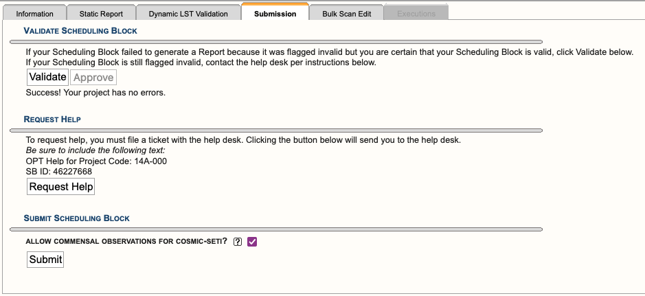 |
|---|
|
Figure 4.7.1: Example of the Submission Tab |
It is important to note here, when the OPT validates an SB it does NOT check the following items:
- allocated science target(s) have been used or have the correct coordinates
- appropriate calibrators have been selected
- correct resource(s) have been selected
- custom resource(s) have been set up correctly, i.e., spectral line
The observer is responsible for correctly setting up their observation(s) and double checking the items listed above. Contact us through the NRAO Science Helpdesk if you have any questions related to SB setup, i.e., need help finding an appropriate complex gain calibrator or advice on the resource setup.
After the SB(s) have been submitted, NRAO staff will check and validate each SB. If we do not find any issues with an SB, it will be approved (changing its status to schedulable — adding it to the dynamic observing queue). Note, we typically do not contact the submitter of valid SB(s). If we do find issues with an SB, we will contact the submitter via the NRAO Science Helpdesk. Please be sure to login to the NRAO Science Helpdesk as least once, so we may find you in the system. To make changes to an SB, you will need to cancel submission (unsubmit).
COSMIC SETI
Starting in the 2023A semester, the COSMIC SETI system came online at the VLA.
The Commensal Open Source Multimode Interferometer Cluster (COSMIC) system is a newly developed digital signal processing instrument deployed at the Karl G. Jansky Very Large Array (VLA), which is designed to enable Search for Extra-Terrestrial Intelligence (SETI) observations to be conducted at the VLA in parallel with "Primary User" PI-led Science observations. The COSMIC system capabilities are still under active development.
To facilitate users not wanting SETI to have access to their data, there is an option to opt-out of this data collection in the Submission tab in the OPT. By default this option is selected to be enabled (checked), unchecking this box will opt you out (Figure 4.7.2). In this case, opting out means that while SETI will still get your raw data, there are no metadata attached to it, e.g., source name, position (RA and Dec), and instrumentation configuration, which renders the received data useless.
 |
|
Figure 4.7.2: COSMIC-SETI opt-out/in checkbox (default is to opt-in, i.e., selected checkbox) |
Cancel Submission
You may cancel submission (Figure 4.7.3) of an SB at anytime if its status is submitted or schedulable. (Note, this is required to make any changes to the SB.) If the SB status is completed or on hold, you may not cancel submission. Contact us via the NRAO Science Helpdesk if you need an SB released from the on hold status.
To cancel submission of an SB:
- select the SB in the left-hand column you wish to unsubmit
- select Submission tab
- select Cancel Submission button
- A pop-up box will appear stating that your SB was successfully cancelled, click Ok.
 |
|
Figure 4.7.3: Cancel Submission (aka unsubmit) |
Linking SBs
Once the scheduling blocks (SBs) are created, you may have some conditional constraints for the execution of their observation(s). Linking SBs is done at the program block (PB) level (as seen in Figure 4.8.1). The PB should contain at least two SBs which are listed with an index number in the first column of the first table in the Scheduling Blocks section.
The concept of linking SBs will allow you to specify alternate SBs within a PB that can be scheduled. For example, in a simple case, you might specify that either SB "1" or SB "2" could be run depending on which LST start range fits best into the schedule. Scheduling priorities are also changed when conditional constraints are specified in a PB. For linked SBs the basic types with their implied priorities are:
| Conditional Constraint | Priority within Linked Blocks | |
| Only one of the blocks | → | LST start range closest to schedule start |
| Total number of executions of the block | → | LST start range closest to schedule start |
| Any of the blocks | → | LST start range closest to schedule start |
| Total hours not to exceed a limit | → | Scheduling Priority Order |
Important Notes
- If an SB is removed (i.e., cut from the left-hand column list), the indexing of the SBs will be re-numbered. Therefore, all linked SBs should be double checked in case the re-numbering of the SB index affected those linked SBs. If those linked SBs received new indexes, then the constraint should be removed and a new constraint be added.
- If a linked SB is unsubmited, the conditional format will be automatically removed. Therefore, be sure to re-link the SBs.
- The SBs within a format statement are evaluated based on the LST start time, with a preference given to the SB in the list that has the earliest SB ID.
- Once a conditional format has been met, the Observation Scheduling Tool (OST) will put the linked SB(s) on hold. Then, we have a cron job that runs every morning around 08:00MT which will expire the SB(s) placed on hold and send an email to the PI, co-I's, and the VLA schedulers. SBs that have been placed on hold and/or expired cannot be selected by the OST for observing.
- Adding no conditions at all, i.e., no linked SBs, is a valid option. We do not require SBs to be linked in order to be considered for observation.
How to Link SBs
To link SBs, select the Edit Constraints button to enter the constraints in the Linked Scheduling Blocks interface above the table of SBs. Constraints are based on the index number of the SB and take the form of selecting those SBs and comparing it to a time or number of execution limit. (Fly-over help is available for all of the fields.)
Once all constraints are satisfactory, the conditions have to be communicated to the system by selecting Stop Editing Constraints. This will notify the on-line system that conditions have been specified and will change the Stop Editing Constraints button into an Edit Constraints button for additional future editing if necessary.
|
|
|---|
|
Figure 4.8.1: Examples of linked SBs. |

Common Examples as Seen in Figure 4.8.1
Observe exactly one of the blocks (1,2)
- This is the most commonly used conditional format. The logic is, observe only one of the two SBs. We often recommend this for observations utilizing two LST start ranges to avoid observing sources transiting too close to zenith.
- Another use case is with multiple SBs so only one of several SBs will be observed. For example, several SBs are created for different weather conditions, i.e., don't run the SB with high-frequency resources when the weather is not suitable, but instead of waiting for the weather to improve, run a different SB with more relaxed weather constraints.
Accumulate blocks (5,6,7,8) to a maximum total of 05:00:00
- This can be used for a set of SBs of varying lengths with appropriate counts/repeats to accumulate a certain amount of time. For example, a 5.0hr SB could be submitted and to help improve chances of getting data, three additional SBs of varying lengths and counts could be submitted and linked to the 5.0hr SB. If the 5.0hr SB is not easily schedulable in the dynamic queue, an accumulation of the shorter SBs could be selected instead.
Observe blocks (9,10,11) to a maximum total of 2 executions
- This is similar to the previous example. Three SBs using different LST start ranges each with a count of 2, yet only 2 executions of this set of SBs should be completed.
Scan Modes and Special Observing Modes
Interferometric Pointing (IP)
Interferometric pointing (a.k.a., reference pointing) may be needed at frequencies of about 15 GHz and higher (K, Ka, Q-band, and most Ku-band setups). At these frequencies the antenna pointing accuracy (a few arcseconds) becomes a significant fraction of the primary beam. Observing with an inaccurate pointing thus may degrade the signal by a significant fraction. The antenna pointing is a function of the shape of the reflective surfaces and is influenced by, amongst other things, gravity and temperature. Therefore, observing at high frequencies may require regular pointing scans to determine offsets from the pointing model. These pointing offsets remain reliable for target sources within about 20d in AZ or EL from the pointing position. Therefore, typically an observation would redetermine pointing solutions when moving to a different portion of the sky, or roughly hourly when tracking a (group of nearby) target source(s).
Pointing scans are performed as a five-point raster observation on a strong (over 300 mJy) continuum calibrator, in first instance in X-band continuum. This primary reference pointing scan usually yields sufficiently accurate pointing offsets, but if more accurate solutions are required a secondary reference pointing may follow at the (standard) frequency of the observing band. Secondary pointing is also performed in continuum mode (to be as sensitive as possible to the continuum source) in an attempt to improve the antenna pointing in the band of interest. However, local lore is that although this might improve the pointing a bit toward the pointing source, subsequent slews and with time passing by, this secondary pointing in general does not yield a long lasting improvement on the primary pointing. In addition, there is the risk that for some antennas the secondary solution fails. The resources for secondary pointing scans are available, but it is debatable whether the extra time spent to perform a secondary pointing scan is worthwhile. Determining pointing solutions using spectral line sources, e.g., with SiO masers in Q-band, has not been tested.
Default pointing resources are included in the NRAO defaults catalog in the group Pointing setups. You may want to copy the X-point (formerly known as the X band pointing) resource and pointing sources you wish to use from the standard catalogs to your personal catalog.
Setting Up an IP Scan
To utilize the interferometric pointing scan mode, select Interferometric Pointing from the drop-down menu under the scan mode section of a scan (Figure 4.9.1a). These scans should use a long enough scan duration (in LST) to include an on source time of at least 2min 30sec. It is advised to start a block of high frequency observations with a pointing scan, and tick the apply reference pointing for each scan thereafter. This tick-box will apply the offsets that were determined in a previous pointing scan; if you forget you will be using the (most likely less accurate) default pointing model. Your first calibrator scan (after the setup scans) may be a pointing scan, but as you don't know in what AZ the array starts, you should allow for ample slewing time or anticipate a worst case scenario using the AZ starting conditions on the Reports tab.
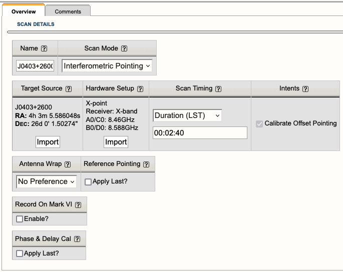 |
|---|
|
Figure 4.9.1a: Example of an Interferometric Pointing scan used in an SB. |
If the pointing scan has not finished by the stop-time of this scan, no valid solutions can be applied. If it has determined a pointing solution before the stop-time has been reached it will continue with another five-point raster, which may or may not yield new solutions (which will be averaged with the first raster solutions). For secondary reference pointing scans, apply the solutions of the preceding primary reference pointing scan.
A pointing scan is for real-time calibration and, while very useful for real-time calibration, usually does not yield useful data for your project. The data is included in the observations, however, you will need special input parameters to load the data in your data reduction package (CASA or AIPS). You may study this data for reference, but the real-time corrections are already applied and cannot be undone.
Tipping (TIP)
Important Note: Currently tipping scans are discouraged since neither CASA or AIPS can apply the results of the tipping scans to the data.
Tipping scans may be needed if you are concerned about calibrating the absolute flux density of your science target source(s). The atmosphere absorbs some of the radiation, and the fraction of the absorbed radiation depends on the opacity, the transparency of the atmosphere. It is mainly dependent on the content of water vapor between the target source and the antenna(s), and can be derived from a series of system temperature measurements at various elevations. An observer would redetermine the opacity on the time scale in which significant changes are expected, i.e., the time scale in which the water vapor content of the atmosphere above the telescopes changes. This is a strong function of baseline length and actual weather and no real guideline on time scales is available.
Tipping scans are performed toward an AZ direction close to your sources at about the observing frequency. The scan samples elevations between about 20 and 60 degrees for a system temperature and can be directed from top to bottom (down) or from bottom to top (up). When you select an AZ for your tipping scan, be aware that shadowing may occur, especially in C and D-configurations. Avoid the AZ directions of the arms, i.e., avoid measuring tips close to the AZs of -5, 56, 115, 175, 236, 295, 355, and 416 degrees.
Setting Up a TIP Scan
To utilize the tipping scan mode, select Tipping from the drop-down menu under the scan mode section of a scan (Figure 4.9.2a). Tipping scans are set up using one of your resources and probably are best done with the widest bandwidth available; make a new resource if you need it. You do not need a physical source. The total duration (LST) of a scan should include the required on source time of 1min 50sec for a tip scan to complete (in one direction, up or down). At the bottom of the page you will have to set the AZ and direction; do not forget this as otherwise you will be slewing to the default AZ of 0d (North) and may hit an antenna wrap constraint/limit. Hitting an antenna wrap limit, can consume half an hour of your observing time to return to your science observing, so always set the AZ.
| Figure 4.9.2a: Example of a Tipping scan. |
You may place any number of tipping scans anywhere in your schedule as you feel fit to monitor the opacity during your observations, although you may want to do this close to your block(s) of high frequency observations. The first scan following the setup scan(s) may be a tipping scan, but as you don't know in what AZ the array starts, you want to allow for ample slewing time or anticipate a worst case scenario using the AZ starting conditions on the Reports tab.
If the tipping scan has not finished by the stop-time of this scan, the data will contain those elevation samples that were completed. If it has completed the tip before the stop-time, it simply will continue with the next scan until the regular stop-time for that scan — this scan may be used to buffer the difference, e.g., absorb the extra time on your bandpass calibrator.
A tipping scan is for post-observation calibration and may or may not yield useful data for your project. The data is included in the observations and you need special switches to load the data in CASA or AIPS. A "tip" would allow you to determine the opacity of the atmosphere during the tipping scan (i.e., during your observation), and you can use that value to correct for the atmospheric absorption in your data.
On The Fly Mapping (OTF)
On the fly mapping or on the fly mosaicking (OTF) scans are different from other scan modes as the data is actually taken with the telescope moving in a scanning motion between two points on the sky. This move is done in a linear fashion with a constant speed with respect to the sky. Note that there currently are two different ways to interpolate over major circles on the sky: one uses Equitorial coordinates (OTFE scans) and the other uses Galactic coordinates (OTFG scans) in the OPT - this is a simple Interpolation Mode toggle in the Scan Mode. Regardless which one is used, the starting and ending coordinates (RA and Dec or Long and Lat) are given in the OPT scan, and the telescope moves in the given stripe direction (see below) at a constant speed linearly in RA/Long and linearly in Dec/Lat. Due to the sky's natural sidereal motion with respect to the telescope, OTF scans from east to west and west to east in principle require different absolute telescope slewing rates seen by the operator, but the slewing rate on the sky is not affected by the direction of the slew. The scan duration, the number of phase center steps, and the number of visibility dumps per integration determine the interpolation mapping grid and map sensitivity as discussed on the mosaicking page of the Observing Guide. Note that these OTF slews are using the Mercator projection of the coordinates in RA/Long and Dec/Lat and therefore might have map deformation implications for OTF close to the (north) Celestial/Galactic pole.
For the remainder of this section it is assumed that the observer has consulted the guidelines given in the mosaicking page, and that the phase center grid and integration time per pointing are known. As OTF modes typically are used to cover a large area of sky in a short time, the default resource integration times are likely to be too long for OTF observations. How to set up an Equatorial OTFE resource is described further below; setting up a Galactic OTFG resource is identical when Long and Lat are substituted for RA and Dec, respectively.
To observe in OTF mode, the OPT needs to know both the beginning and end points of the OTF scan in J2000 Right Ascention (RA) and Declination (Dec) or in Galactic Longitude (Long) and Galactic Latitude (Lat). The scan from the beginning to the end point is referred to as a "strip" or "stripe". Per strip these two boundary target positions must be defined in the source list (SCT) as two distinct sources. The intermediate phase centers for the mapping between the beginning and end points are determined by the on-line system as described below. These intermediate points are not displayed in the Reports tab of the SB, only the boundary positions. Of course these boundary target points can be entered in the SCT manually, but for any larger (rectangular, hexagonal, etc) grid mosaic, by far the easiest way to define sources in the SCT is to generate the grid of boundary points (e.g. pairs of RA values with each pair having the same Dec) using a text editor and to import this grid with the text import tools given under the Source Lists section of Text Files and Catalogs in the OPT. Some examples are given below; boundary points provided in coordinates other than equatorial will be converted to J2000 RA and Dec internally by the SCT (i.e., also for the Galactic coordinate version, but this will be opaque to the observer).
Setting Up an OTF Scan
To utilize the OTF scan mode, select On The Fly Mapping from the drop-down menu under the scan mode section of a scan (Figure 4.9.3a). For stripes interpolated in the J2000 frame, leave the default Interpolation Mode as Equatorial. Switching to the Galactic interpolation mode instead will do the same as the Equatorial version with the difference that it will interpolate in Galactic coordinates - the rest is essentially the same and therefore the below will only highlight the Equatorial version. Selecting this scan mode reveals the required fields to schedule an OTF strip. These fields are not only the beginning and ending position of the strip (as defined above), but also some specific settings for defining the strip. The number of steps and the integrations per step both require user input. The value for integration time is provided from the selected "hardware setup" resource, whereas the stripe duration is equal to the number-of-steps-plus-one multiplied by the number-of-integrations-per-step, then multiplied by the integration time. The plus-one is added to the number of steps to account for the time required for the telescope to reach the appropriate constant speed. (The telescope actually begins its motion from just beyond the boundary point, in order to be in motion at the appropriate scanning speed from the starting point for the OTF scan. The time for this speed build-up results in an extra "step" that will be flagged in the visibility data). Note that the stripe duration is not the same as the scan timing duration. The latter should include at least 10-15 seconds of additional overhead to position the telescopes for the beginning of the strip (e.g., to include turn around and settle time) and thus somewhat depends on the angular distance to slew between the observed strips.
 |
|---|
|
Figure 4.9.3a: Example of an OTFE scan from a VLASS scheduling block. |
|
OTFE Mode Dependent Settings |
|
|---|---|
|
Number of Steps (variable N) |
The strip is divided linearly in N-1 equal parts between the RA end-points, and similarly in Dec, and thus contains N pairs of (RA,Dec), including the end points. These coordinates will constitute the phase centers used during the strip observation and end up as the "sky target positions" (or mapping grid points) of the data taken along the strip in the visibility data set. Each of these RA,Dec coordinates (fields) can be individually imaged if desired, or selectively included in joint deconvolution algorithms. |
|
Integrations Per Step (variable M) |
This is the number of time intervals associated with each phase center, i.e., each RA,Dec coordinate above. If individually imaged, the total integration time per field is M*Tvis (see next) and thus a measure for the image sensitivity (but see the mosaicking page for more accurate details). |
|
Integration Time (Tvis) |
This is the integration time per visibility as specified in the resource selected in the resource field. |
|
Stripe Duration (Tstrip) |
The time it will take to complete this strip observation. The time includes the extra startup integration for the strip (i.e., N+1 steps), but excludes the overhead time for slewing the telescopes to the starting location for the strip. This number is calculated as: Tstrip = (N+1)*M*Tvis |
|
Scan Timing (Tscan) |
The total time of the scan, input by the user, which must account for the Stripe Duration time plus slewing overhead from the previous telescope location (e.g. the end source of the previous scan) to the starting location for this scan. The slewing overhead should include at least 10-15 seconds if the scan is the continuation of a previous strip pattern (e.g., a reversal of the motion at the next strip in the same area of the sky), but otherwise may need significantly more extra time if it is the first strip of a new mosaic (e.g., if the previous scan was on a complex gain calibrator or some other source that is not part of the OTF scanning). Therefore this number should be at least Tscan > Tstrip + 10sec. See the scan import example below. |
|
Remaining Overhead |
This value is equal to "scan timing" minus the "strip duration", and thus reports the additional overhead time for the scan. Observers should ensure that this value is at least 10-15 seconds in order to allow for slew time from the end of the previous scan to the start location for this OTF scan, as well as to allow for settling time. |
|
Select RA Direction |
Moving between two positions on the sky can be done in several ways: decreasing in RA, increasing in RA, or the shortest direction. The default is to choose the shortest direction in RA (and always the shortest direction in Dec). However, the direction of motion in the RA direction can be explicitly selected using the radio buttons here. Of course, when going the long way instead of the short route, the on-the-sky slew rate calculation below should use the strip angle of the longer path. |
The on-the-sky slew rate is determined by the strip angle (in arcmin or arcsec) and the stripe duration (in minutes or seconds), where the maximum tested slew rate in S-band currently is of the order of 10 arcmin per second, which is the same as 10 degrees per minute:
slew rate = (Change in angle)/(N*M*Tvis)
As for standard scan modes, the data rate is determined by the resource details. That is, as determined by the amount of correlator capacity used and by the dump time (Tvis). The resource summary in the RCT will show this number when creating the resource, and the reports summary page top table will also summarize it. Note that for the typically short integration times used in OTF, the data rate quickly will approach or exceed the limits set for General Observing Capability modes.
Create an OTF Resource
The main difference between a normal observing scan resource and an OTF resource is that typically the visibility dumps should occur at a faster rate than the potential smearing effects on the data. It is thus advisable to dump at least a few times while the telescopes move a primary beam on the sky, say Tvis(sec) <~ 0.1 x freq(GHz) / slew-rate(arcmin/sec), but this is dependent on the required sensitivity and science goal. Detailed guidance is provided in the mosaicking page of the Observing Guide
The resource can be created as described in the OPT RCT section, with the visibility integration time entered in the first tab. However, care should be taken not to exceed the current data rates (shown in the box in the RCT), which happens easily with demanding correlator setups as well as with shorter integration times.
Current constraints:
- Phase centers (N) cannot be changed faster than at 0.5 second intervals.
- Visibility integration (dump, Tvis) times must be at least 250 ms (which would be the integration time in the RCT).
- Resource data rates may not exceed the limits for (Resident) Shared Risk as stated in the current OSS.
- Limited slew rates in Azimuth (40 deg/min) and Elevation (20 deg/min) will pose a limit on the maximum slew rate in RA and Dec, depending on geometry (and LST) of the observation. It is best to stay on the safe side of these limits.
Additional Notes
- Slewing at high elevations should be minimized due to potential tracking and dish deformation issues close to zenith. That is, for OTF targets close to 34 deg Dec, map well before or well after transit, i.e. close to rise or set!
- When scanning in Galactic coordinates being close to Dec 34o may not be obvious; check your Declinations!
- Times for dumps are in UTC (which is very close to LST for Tvis << 1 min), scan times are in LST.
- Individual antennas may start and stop scanning a strip up to 0.5 seconds late with respect to the rest of the array. This discrepancy will introduce a pointing offset of up to 0.5(sec) x slew-rate for that antenna. To limit imaging problems without flagging such antennas as bad (where one may known which antennas were affected), observers should keep the offset smaller than about 1/4 of the primary beam FWHM, as calculated at the highest frequency in the observing band, when planning for potential slew-rates.
- See mosaicking page for Tvis and other mosaicking hints.
Examples
Suppose we observe in X band and follow the mosaicking web page to get the sampling distances in Equatorial coordinates, i.e., we assume an observing frequency of 9.33 GHz and hexagonal packing at sqrt(3) which is almost the same as using the upper part of the band and sqrt(2). The primary beam is thus 4.5 arcmin (270 arcsec) and we use a strip separation of 2.6 arcmin (156 arcsec). Remember that (ΔRA in angle) is (ΔRA in time) multiplied by 15 × cos(Dec), e.g. 4min at 60d = 4min x 15'/min x cos(60d) = 30 arcmin; similar for Galactic coordinates where ΔLong is multiplied by cos(Lat).
The minimalistic SCT input files then may look like this (see text-file input):
1a. A 20-arcmin length, 4-row (10' wide) rectangular area scanned in RA (constant Dec) centered on (J2000) RA=12:00:00, Dec=00:00:00
row01west ; ; ; ; 11:59:20; +00:03:54; ; ; ; ;
 row01east; ; ; ; 12:00:40; +00:03:54; ; ; ; ;
row02west ; ; ; ; 11:59:20; +00:01:18; ; ; ; ;
 row02east; ; ; ; 12:00:40; +00:01:18; ; ; ; ;
row03west ; ; ; ; 11:59:20; -00:01:18; ; ; ; ;
 row03east; ; ; ; 12:00:40; -00:01:18; ; ; ; ;
row04west ; ; ; ; 11:59:20; -00:03:54; ; ; ; ;
 row04east; ; ; ; 12:00:40; -00:03:54; ; ; ; ;
1b. A 20-arcmin length, 4-row (10' wide) rectangular area scanned in RA (constant Dec) centered on (J2000) RA=12:00:00, Dec=+60:00:00
row01west ; ; ; ; 11:58:40; +60:03:54; ; ; ; ;
 row01east; ; ; ; 12:01:20; +60:03:54; ; ; ; ;
row02west ; ; ; ; 11:58:40; +60:01:18; ; ; ; ;
 row02east; ; ; ; 12:01:20; +60:01:18; ; ; ; ;
row03west ; ; ; ; 11:58:40; +59:58:42; ; ; ; ;
 row03east; ; ; ; 12:01:20; +59:58:42; ; ; ; ;
row04west ; ; ; ; 11:58:40; +59:56:06; ; ; ; ;
 row04east; ; ; ; 12:01:20; +59:56:06; ; ; ; ;
2. A 7-point (3-row, ~8' diameter) hexagonal scanned in RA (constant Dec) centered on (J2000) RA=12:00:00, Dec=00:00:00
row01west ; ; ; ; 11:59:49.6; +00:02:36; ; ; ; ;
 row01east; ; ; ; 12:00:10.4; +00:02:36; ; ; ; ;
row02west ; ; ; ; 11:59:39.2; +00:00:00; ; ; ; ;
 row02east; ; ; ; 12:00:20.8; +00:00:00; ; ; ; ;
row03west ; ; ; ; 11:59:49.6; -00:02:36; ; ; ; ;
 row03east; ; ; ; 12:00:10.4; -00:02:36; ; ; ; ;
3. A 14-point (5-row, ~13' diameter) hexagonal scanned in RA (constant Dec) centered on (J2000) RA=12:00:00, Dec=+60:00:00
row01west ; ; ; ; 11:59:39.2; +60:05:12; ; ; ; ;
 row01east; ; ; ; 12:00:20.8; +60:05:12; ; ; ; ;
row02west ; ; ; ; 11:59:18.4; +60:02:36; ; ; ; ;
 row02east; ; ; ; 12:00:41.6; +60:02:36; ; ; ; ;
row03west ; ; ; ; 11:58:57.6; +60:00:00; ; ; ; ;
 row03east; ; ; ; 12:01:02.4; +60:00:00; ; ; ; ;
row04west ; ; ; ; 11:59:18.4; +59:57:24; ; ; ; ;
 row04east; ; ; ; 12:00:41.6; +59:57:24; ; ; ; ;
row05west ; ; ; ; 11:59:39.2; +59:54:48; ; ; ; ;
 row05east; ; ; ; 12:00:20.8; +59:54:48; ; ; ; ;
Example SB
An example of an SB that can be created with a text editor and imported in the OPT using the third example, may look like this (see explanation of the fields):
# example SB for OTF in equatorial coordinates on W51
#
VERSION; 3;
#
# rectangular Equatorial-OTF in S band, 8 strips, 0.5s
#
# define catalogs in which Sources and Resources can be found by name
 SRC-CAT; OTF, VLA;
HDWR-CAT; OTF, NRAO Defaults;
# Scheduling Block details
SCHED-BLOCK; OTF_W51_S; Dynamic; 1; 2014-06-07; 16:00:00-21:00:00 ; 25.0; D; 225.0; 35.0; N; N; w=100.0,p=60.0; ;
#
# startup scans on calibrators
 STD; Dummy; 3C286_S; S16f_otf_0.5; DUR; 1m; cw; N; N; N; N; SetAtnGain,; ;
 STD;3C286;3C286_S; S16f_otf_0.5; DUR; 9m; cw; N; N; N; N; CalFlux, CalGain, CalBP; ;
#
# Slew to calibrator close to mapping area
# slew from calibrator to beginning point of mapping row 1
# first 4 rows of map
 STD;J1925_S; J1925_S; S16f_otf_0.5; DUR; 6m; ; N; N; N; N; CalGain,; ;
 STD;Setup01; row01left; S16f_otf_0.5; DUR;35s; ; N; N; N; N; ObsTgt,; ;
 OTFE; row01; row01left; row01rght; S16f_otf_0.5; DUR; 144s; 32; 8; 0; ; N; N; N; N; ;
 OTFE; row02; row02rght; row02left; S16f_otf_0.5; DUR; 144s; 32; 8; 0; ; N; N; N; N; ;
 OTFE; row03; row03left; row03rght; S16f_otf_0.5; DUR; 144s; 32; 8; 0; ; N; N; N; N; ;
 OTFE; row04; row04rght; row04left; S16f_otf_0.5; DUR; 144s; 32; 8; 0; ; N; N; N; N; ;
#
# Slew to calibrator
# slew from calibrator to beginning point of mapping row 5
# next 4 rows of map
# final calibrator scan
 STD;J1925_S; J1925_S; S16f_otf_0.5; DUR;95s; ; N; N; N; N; CalGain,; ;
 STD;Setup05; row05left; S16f_otf_0.5; DUR;35s; ; N; N; N; N; ObsTgt,; ;
 OTFE; row05; row05left; row05rght; S16f_otf_0.5; DUR; 144s; 32; 8; 0; ; N; N; N; N; ;
 OTFE; row06; row06rght; row06left; S16f_otf_0.5; DUR; 144s; 32; 8; 0; ; N; N; N; N; ;
 OTFE; row07; row07left; row07rght; S16f_otf_0.5; DUR; 144s; 32; 8; 0; ; N; N; N; N; ;
 OTFE; row08; row08rght; row08left; S16f_otf_0.5; DUR; 144s; 32; 8; 0; ; N; N; N; N; ;
 STD;J1925_S; J1925_S; S16f_otf_0.5; DUR;95s; ; N; N; N; N; CalGain,; ;
#---END---
Solar (SOL)
The Solar (SOL) observing mode is only utilized for a solar target, that is a location near or on the solar disk. This section will focus on how to setup solar source(s) in the SCT and how to use the SOL scan mode in the OPT. For more details on solar observing and how to setup a solar SB in the OPT, refer to the Solar Observing section of the Observing Guide.
Create a Solar Source
Before creating the observation, the observer must first create solar source(s) in the SCT. Since the Proposal Submission Tool (PST) cannot anticipate the solar target of interest, the observer’s source will not appear in any existing catalog and the observer must create one under the SCT.
To add a source to the catalog, click on FILE → CREATE NEW → SOURCE (see Figure 4.9.4a).
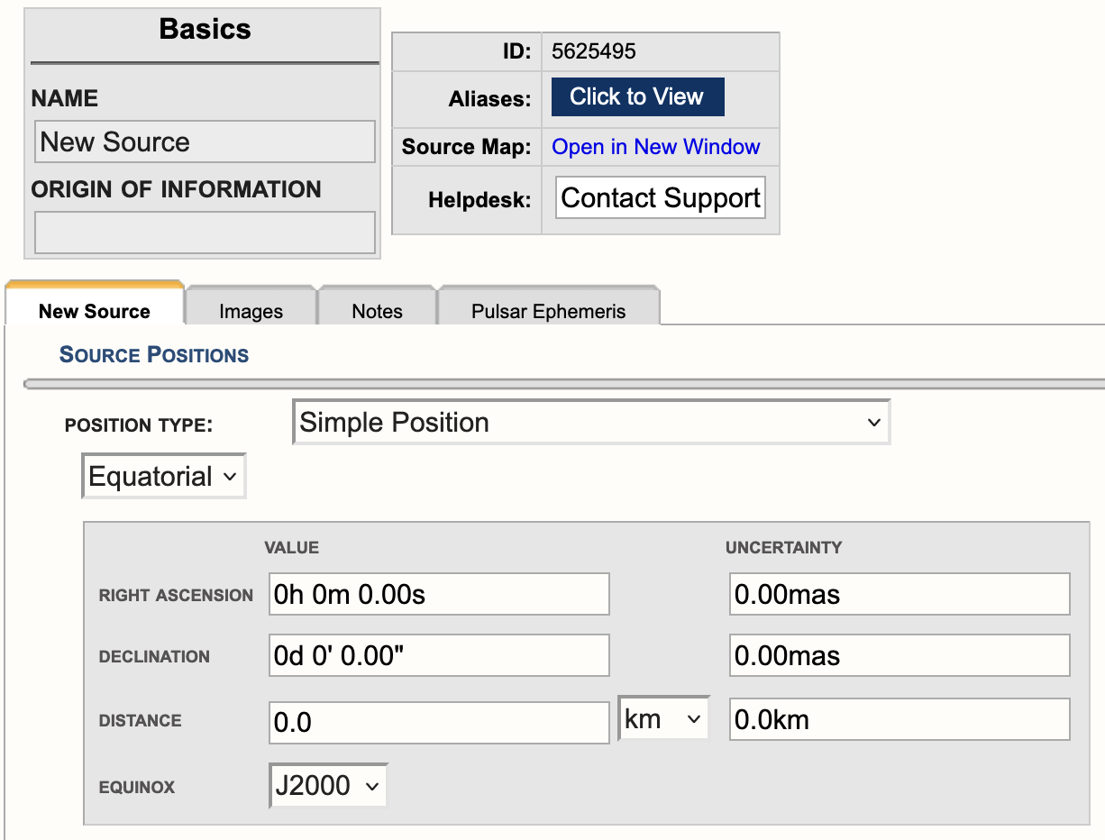 |
|---|
|
Figure 4.9.4a: Screen cap of a new source in the SCT. |
Under the Source Positions field click on the pull-down menu to the right of Position Type and select Solar System Body with Uploaded Ephemeris (see Figure 4.9.4b). For more information regarding the ephemeris, refer to the Solar Observing section of the Observing Guide.
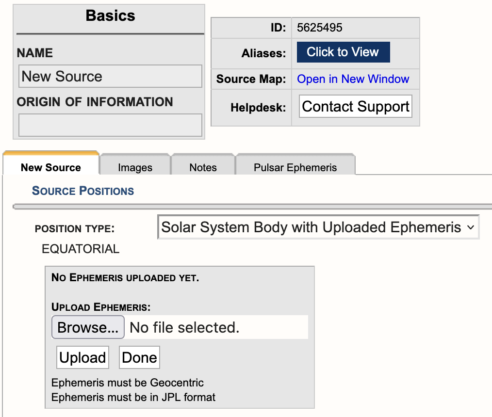 |
|---|
|
Figure 4.9.4b: Screen cap of new source position type Solar System Body with Uploaded Ephemeris. |
Click on Browse to select a solar target ephemeris and then click Import. Note that the ephemeris must be geocentric and must be in JPL format. Enter a Name for the ephemeris target and, if necessary, repeat the process to enter additional targets into the catalog.
Setting Up a Solar Scan
Now that you have created the solar source(s) for the observation and assuming the resource has also been created in the RCT per the approved proposal. The next step is to create a solar observing scan in the SB.
To utilize the solar scan mode, select Solar from the drop-down menu under the scan mode section of a scan (Figure 4.9.4b). This enables an additional pull-down menu at the bottom of the page under Mode Dependent Settings. The table below describes the parameters in detail and which to utilize.
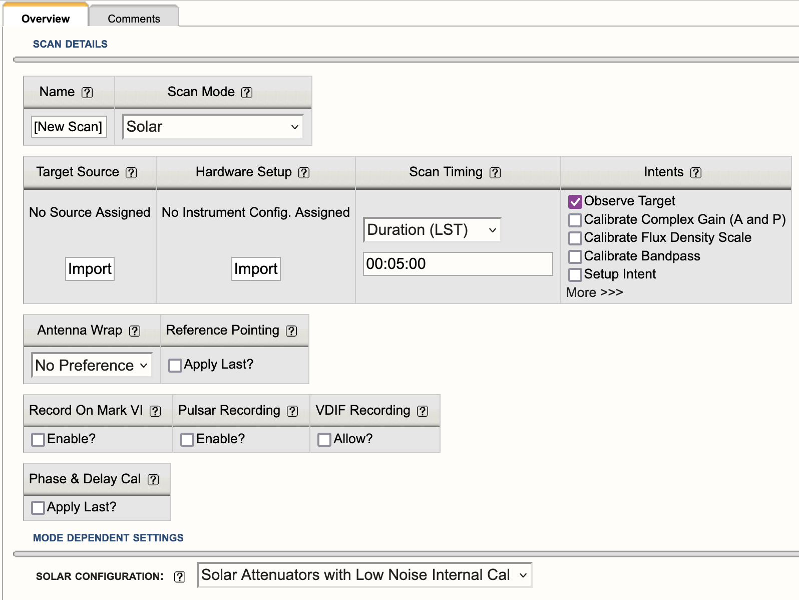 |
|---|
|
Figure 4.9.4c: Example of a Solar scan mode. |
|
Solar Mode Scan Details |
|
|---|---|
| Target Source |
Import the target position you have defined as a solar source in the SCT. |
| Hardware Setup |
Import a resource in one of the observing bands that are capable of performing solar observations (one of the bands covering 1-18 GHz plus the 230-470 MHz band). |
| Mode Dependent Settings |
Solar Configuration: This setting must be used to insert the special attenuators to ensure that the signal from the Sun is manageable and that appropriate switched cal signals are employed.
|
Pulsar Observing Modes
The VLA supports two different types of pulsar observing:
- Phase-binned imaging mode, in which visibility data are averaged into a number of bins corresponding to different rotational phases of the pulsar. This allows, for example, separate imaging of on-pulse and off-pulse portions of the data.
- Phased-array pulsar mode (also called YUPPI mode), in which antenna data streams are coherently summed in order to produce a high-time-resolution, single-pixel data set. The data can optionally be folded in real-time using a pulse period ephemeris.
Either mode can be configured via the Pulsar tab when creating an instrument configuration in the RCT. For modes that require one, a Tempo-compatible period ephemeris file should be attached to each source in the SCT. Additional information about setting up these modes can be found in the pulsar section of the Observing Guide, and in the OSS pulsar section. If you have questions not addressed in these documents, please contact us through the NRAO Science Helpdesk.
Subarray Observing
The 27 VLA antennas can be used in subsets, to observe several independent programs simultaneously. Typical uses are to observe different sources that are bright enough that not all antennas are needed for the full sensitivity, or observing the same source at different observing bands at exactly the same time.
Subarray Guidelines
When preparing for subarray observing, all procedures, advice, and restrictions to create Scheduling Blocks (SBs) should be followed, as described in the previous sections of the manual. Any source and most resources available in the SCT or RCT catalogs, respectively, can be used in creating scans for the subarray. There are no restrictions in sources, scan intervals, scan timing, pointing scans, etc., between the subarrays other than the general limits, including restrictions for General Observing programs (i.e., up to three independent subarrays using standard 8-bit and 3-bit continuum setups and no special modes such as pulsar, OTF, etc., as that would make it a (Resident) Shared Risk program). There are restrictions in the division of antennas over the subarrays; in particular three subarrays of nine antennas each is not allowed. Further details on using subarrays can be found in the VLA Observing Guide and the Observational Status Summary (OSS).
Summary
- Subarray observing should be proposed for and be approved by the TAC.
- Subarray observing is General Observing and has restrictions accordingly; e.g., only standard observing with 8-bit and/or 3-bit continuum resources from the NRAO default list. Other modes or more than 3 arrays are in the Shared Risk categories.
- A division in three subarrays is typical one of 11, 8 and 8 antennas on the array; a division in two usually has 15 and 12 antennas per subarray allocated. Typical subarray antenna distributions over the whole array are homogeneous, random, or the inner antennas for the higher frequencies in a subarray and the outer for the lower frequency bands in another subarray. The latter is done to attempt to get a similar angular resolution between the observing frequencies.
- Subarrays cannot be generated with text-file uploads of SBs. However, if the Subarray Loop structure is in place, text-file scan lists can be imported in each subarray Loop separately (File → Import Scans...).
We are working on creating the three Reports separately for each Subarray Loop in an update of the OPT, but for now only the Schedule Summary Report (located at the bottom of the Reports tab of an SB) shows independent information per Subarray Loop.
How to Create Subarrays
Currently, creating a subarray schedule in the OPT is implemented by the use of scan loops with different scans (e.g., different sources, or the same sources with differing resources), where the loops are executed at the same time with different subsets of antennas. This is not the optimum implementation and we are working on a better scheme for the future. For the moment please follow these instructions:
- In the Program Block (PB) created for the project and approved for subarray observing, create a Scheduling Block (SB) if it is not already present. The details such as LST start range, weather conditions, count, etc., entered for this SB will apply to all of the subarrays created within the SB.
- To create a subarray in the SB, select the SB and make sure the SB is empty, i.e., no scans, then, select File → Create New → Subarray.
- To create additional subarrays within the same SB, select the newly created Subarray Loop and then select File → Create New → Subarray. Up to three subarrays can be created for General Observing.
- Divide the array into subarrays, per Subarry Loop (see Figure 4.9.6a).
- Tick the boxes of stations that should make up the subarray configuration.
- Already used antennas should not be selectable. Note that the numbering is from the center of the array (#1) out to the furthest one on the arm (#9), where N, E, and W stand for the North, East, and West arms, respectively. The allocated array configuration is specified in the PB; the actual antenna pad numbers scale with the principal array configurations (Any, A, B, C, D) but the order specified in the Subarray Loop is in which order the antennas are allocated on each arm per subarray.
 |
|---|
|
Figure 4.9.6a: Example of three subarrays under an SB. |
- Create your Scan Lists in each of your subarrays.
- Scan loops are allowed. Copying scans from one subarray to the next should work as usual, etc. However, do not use the tick-box Keep Previous Configuration under the Instrument Configuration for the first scan resource in your subarray. Make sure the total time per Subarray Loop adds to (almost) the same time, as otherwise the shorter subarrays will be idling while the longest has to finish (and which total time will count toward your allocated time).
- Once each Subarray Loop contains valid scans, the Reports page of the SB can be used to generate resource, source, and scan summaries. However, as a WARNING at this time, the Reports summaries include all resources and accumulated time on source over the subarrays. That is, all resources used in any Subarray Loop is listed in a single Resource Summary table. Also, if a source/resource/intent combination appears in more than one Subarray Loop, the total number of scans and total accumulated time is listed in a single Source Summary Table. However, when unfolding the loops in the Scan Listing table, they do list the scan listing per Subarray Loop correctly in the loops, i.e., each loop starts at the same LST to show the scan timings, elevations, etc., of the scans in each subarray. Check the end times of each of the loops to make sure they do not differ too much.
- Validate and submit the SB when done. Be sure to disable COSMIC-SETI. This is necessary only for subarray observations.
VLA + LWA Observing
Disclaimer: Non-standard eLWA observing is currently listed as RSRO (Resident-Shared Risk Observing) and not GO (General Observing). A fixed version of this mode is available as Shared Risk Observing as of semester 2022A and available from the list of default setups, labeled as "eLWA (from semester 22A)". If you have questions regarding eLWA observing, please contact us through the NRAO Science Helpdesk.
VDIF stands for VLBI Data Interchange Format and was introduced in 2009 to standardize data transfer and storage for Very Long Baseline Interferometry (VLBI) observations. The expanded Long Wavelength Array (VLA + LWA = eLWA) observing mode uses this format to record a VDIF data stream for each VLA antenna. The VDIF files are then combined with raw voltage beam data from the New Mexico Long Wavelength Array stations and are correlated offline using a software correlator after the observation is completed.
The Fundamental Steps for Creating an eLWA SB
Step 1: Create VDIF Instrument Setup
First, go to Instrument Configurations (RCT), select the resource catalog you wish to create a new resource, and select FILE → CREATE NEW → 8-BIT INSTRUMENT CONFIGURATION.
- Basics tab: Give the resource a name, e.g., VDIF 8 MHz, then select the receiver band 4 (54.0 - 86.0 MHz). The correlator integration time in this case is not relevant, just specify 5.0 seconds.
- Basebands tab: Set the center frequencies to 536.0 MHz.
- Subbands tab: Add one subband, select 8 MHz bandwidth, put BB_center-460.0 MHz to set central frequency to 76 MHz, and then set polarization to Dual and Recirculation to 1x.
- Special Modes tab: Select the VDIF tab and select Yes for Recording.
- Validate tab: Make sure the summary looks like Figure 4.9.7a shown below and no validation errors are reported.
 |
|---|
| Figure 4.9.7a: Validation page in the Resource Catalog Tool (RCT) of a valid VDIF resource. |
Step 2: Enable scan for VDIF recording
When creating a new scan, select the above created VDIF instrument configuration. In order to enable VDIF recording, you also need to set the checkbox for VDIF Recording within the scan and it is also strongly recommended to disable the 10 Hz switched power, by selecting the Disable checkbox. Your scan should look similar to the example in Figure 4.9.7b below.
 |
|---|
| Figure 4.9.7b: Example of a scan using VDIF recording. |
Important Note: If you plan to trigger resetting requantizers using a setup scan and the VDIF recording instrument configuration, then 10 HZ SWITCHED POWER must be unchecked, to have switched power enabled, and VDIF RECORDING should be disabled by leaving it unchecked.


Text Files and Catalogs in the OPT Suite
Text Files
Apart from direct manual editing in the fields exposed by the web interface, all components of the OPT Suite (i.e., OPT, RCT, SCT) can import and export ASCII text files that, e.g., can be created and manipulated or optimized by computer programs or scripts outside the OPT Suite.
A source list can be prepared from external source catalogs and formatted such that the SCT can ingest it, or a source list can be exported to a text file. Similar catalog operations can be performed on resource catalogs as well. Furthermore, (re)source lists can be extracted from an existing scheduling block and can be shared or loaded in either the RCT or the SCT. The OPT can read and write scan lists or ingest script-generated scheduling blocks, etc.
This section describes the syntax that might be of interest to most users of this feature: importing source lists into the SCT and importing scan lists or complete scheduling blocks into the OPT. A properly formatted standardized list of spectral lines is also provided for upload. To be able to read in scans or scheduling blocks into the OPT without overloading the individual entries with too many variables, the source and resource catalogs must be defined beforehand (so that the scan parser can grab the (re)source definitions from the existing catalogs). If only VLA calibrators and NRAO default resources are required, no other additional (re)source catalogs need to be defined.
The following sections in this section of the OPT manual describe the syntax for importing source lists into the SCT, naming resources in the RCT, and for importing scan lists and scheduling blocks into the OPT. For information about importing source lists into the Proposal Submission Tool (PST), see the Sources section of the Proposal Submission Guide. RCT resources, but only in XML format, are imported similarly.
General Syntax
The import of text files is accomplished by parsing each line, where each line is assumed to define a complete instruction. Parsing occurs for plain ASCII characters so if a rich-text capable text editor is used (e.g., Word) please save without rich-text formatting in plain ASCII text or the import will fail without an error message. Empty or whitespace-only lines and lines where the first non-whitespace character is a hash (# symbol) are ignored. That is, hashes may be used to insert comments in the text file. Typical lines will have input fields delimited by semi-colons (;), where multi-variable fields have their variables separated by commas (,). The comma after the final value of a field is optional, but the final semi-colon after the final field is mandatory (except for spectral line lists). Leading and trailing whitespace around field variables is ignored, but whitespace between the first and last non-whitespace character of a variable is preserved (see examples). Optional fields may be left unspecified (i.e., no characters or whitespace-only characters) and will be assigned a default value where appropriate. Character fields are treated as case-sensitive unless otherwise specified. Prohibited characters in (free-format text) fields are non-printable (tab) characters, including any form of end-of-line characters, variable delimiters (semi-colon and comma), and any of the specified ones in the table below; leading and trailing whitespace around free-format text variables is ignored, but whitespace within freeformat text is preserved.
The full list of acceptable and prohibited characters in free-format text fields in the OPT Suite is given in the table below. Note the differences of accepted characters when using the VLA CASA Pipeline (prohibited characters would not appear in the data processing stage when the OPT is used); it may be best to avoid OPT Suite accepted characters (only) in observer and source names that are not accepted by the VLA CASA Pipeline, i.e., [ and ] nor #, and probably also parentheses:
| OPT Suite acceptable characters* | VLA CASA Pipeline notes (if different from OPT Suite)** | ||
|---|---|---|---|
| a-z A-Z | lower and upper case letters | ||
| 0-9 | digits | ||
| spaces | |||
| + - . = | plus, minus, period/decimal, and equal signs | ||
| / _ # * | slash, underscore, hashtag (octothorpe), and asterisk | does not accept # in Flux cal name, but does accept # in observer and other source names | |
| ( ) [ ] | open/close parentheses and square brackets | does not accept [ nor ] in any source name, but does accept [ and ] in observer name | |
| OPT Suite prohibited characters | |||
| ' " | single quote and double quote | accepts " in observer name and ' in observer and any source name | |
| { } | curly brackets | accepts { and } in observer name | |
| < > | less than and greater than | ||
|
end-of-line and non-printable characters (e.g., "tab"), rich-text formatted text or other non-ASCII characters |
accepts "tab" at the end of observer name |
||
| \ @ % $ | backslash, at, percent and dollar signs | accepts \ in observer name and @ $ % in observer and source name | |
| ` ~ ! ^ & | : , ; ? | other textual and linguistic characters | accepts , in observer name and ` ~ ! ^ | : ; ? in observer and source name |
*) Anywhere in the text file that is uploaded, including Scheduling Block name, User Comments/Notes, etc.
**) Some characters (parentheses and most characters in the bottom row) used in the VLA CASA Pipeline (especially in the Phase calibrator name) may cause several of the plots in the plotsummary stage to differ slightly from when these characters do not appear in source names. This causes the numbers in the makeimages task to differ slightly as well.
SCT: Importing Source Lists
Syntax
Text files with source lists can be imported into the SCT if they use the following syntax. Note that this is the same format as for the PST, so if you have uploaded your source list into the PST, you can use the same file for uploading in the SCT. Every line containing any source information in the file must define a separate source as:
sourceName;groupNames;coordSystem;epoch;longitude;latitude;refFrame;convention;velocity;calibrator;
The text file should only contain lines formatted as above, or lines that are known to be ignored by the parser (i.e., empty or whitespace-only lines and comment lines starting with an # (octothorpe)). An (optional) exception is if the very first line is starting with an * (asterisk); the string after the asterisk will replace the default source catalog name, where a leading space in the string is ignored. Start with the catalog name syntax line before any source syntax line or any comment line or this source catalog name will not be picked up (and an "[Unnamed Catalog]" results):
* Source catalog name in the SCT
# this is a line with a comment and the previous line is the syntax used to include all sources into a non-default
# (the catalog name line will be ignored by the PST when uploading this file)
# the rest of the source list file contains source lines mandated as above and other ignored lines
<source1 line>
<source2 line>
...
Every data line must have ten semi-colons (;), including the one after the final calibrator field; note that the catalog name line, the one starting with the asterisk, should not contain any semi-colon.
Details and possible (predefined) values per field are described in the table below.
| sourceName |
Mandatory, single value
|
| groupNames |
Optional, unlimited number of comma-separated values
|
| coordSystem |
Optional, single value (defaults to equatorial), not case-sensitive
|
| epoch |
Optional, single value (defaults to J2000), not case-sensitive
|
| longitude |
Mandatory, single value
|
| latitude |
Mandatory, single value
|
| refFrame |
Mandatory in combination with convention and velocity, single value, not case-sensitive
|
| convention |
Mandatory in combination with refFrame and velocity, single value, not case-sensitive
|
| velocity |
Mandatory in combination with refFrame and convention, single value
|
| calibrator |
Optional single value (defaults to N), not case-sensitive
|
To ingest a text file with a source list, navigate to the SCT. Select from the menu FILE → IMPORT and then select PST for the import format. After providing a file to import, a new catalog with the default name [Unnamed Catalog] will be created. If the imported sources need to be included in a different catalog, or a different catalog group, use the general copy/paste method of the web application to move the sources around. Alternatively, change the name of the new unnamed catalog in the SCT using the Properties tab of that catalog if a name was not specified with an * (asterisk) line.
Source List Examples (in SCT/PST format)
Minimalist: Source name and coordinates only, default coordinate system, epoch and unspecified velocity.
J0433+0521;;;;04:33:11.095535;05:21:15.619420;;;;;
J1119−0302;;;;11:19:25.3;−03:02:51.32;;;;;
<some_name> <4 times ";"> <RA_j2000> ; <Dec_j2000> <5 times ";">
Explicit: Same data as minimalist, above, but with coordinate system and epoch stated in long form, and spaces for ease of reading.
J0433+0521; ; equatorial; J2000; 04:33:11.095535;  05:21:15.619420; ; ; ; ;
J1119−0302; ; equatorial; J2000; 11:19:25.3     ; −03:02:51.32    ; ; ; ; ;
Full: All fields are specified, starting by naming the catalog MyPrivateList in which these sources should appear (instead of the default Unnamed Catalog); multiple values in those fields that allow it, with spaces in source and group name, some case-preserved and case-ignored variable names, and with optional trailing comma in velocities.
* MyPrivateList
# This is my private list of secret sources..
Secret Source; My Recipes, Private; equatorial; J2000; 12:34:56.789; 87.65432; lsR; Optical; −98.6,; y;
RCT: Importing Spectral Line Lists
Syntax
The RCT uses rest frequencies and corresponding spectral line definitions when attempting to set up the WIDAR correlator and populate the subbands in the basebands. Filling out the line parameters takes some effort and has to be repeated for each new resource. Therefore, in the resource lines tab in the RCT, it has a feature to export and import line definitions using plain (editable) text files. Note that the main intended use is to export lines from one resource to import in another, not to create one from scratch (we give no guarantees that it will be parsed properly in that case). Another item to note is that the source position for Doppler setting is not retained in the text file export and thus cannot be defined for text file import. Note that we created a template at the bottom of this page.
Every line containing any spectral information in the file must use the following syntax:
lineName;restFreq;refFrame;convention;velocity;velRange;velSep;polProd;other
The text file should only contain lines formatted as above, or lines that are known to be ignored by the parser (i.e., empty or whitespace-only lines and comment lines starting with a #-hash). Every data line must have eight semi-colons (;), which means that there is none after the final field. Multi-value fields use commas as item separators.
Details and possible (predefined) values per field are described in the table below.
| lineName |
Mandatory, single value
|
| restFreq |
Mandatory, single value larger than zero, unit defaults to GHz
|
| refFrame |
Mandatory, single value, not case-sensitive
|
| convention |
Mandatory, single value, not case-sensitive
|
| velocity |
Mandatory, single value, unit defaults to km/s
|
| velRange |
Mandatory, single value larger than zero, unit defaults to km/s, value defaults to 100 (i.e., 100.0km/s)
|
| velSep |
Mandatory, single value larger than zero, unit defaults to km/s, value defaults to 1 (i.e., 1.0km/s)
|
| polProd |
Mandatory, multi-value, not case-sensitive
|
| other |
Optional, multi-value, not case-sensitive
|
To export a line list from a resource, navigate to the lines tab for the resource in the RCT. At the bottom of the tab, use the Download Spectral Lines button. Similarly, use the Import Spectral Lines button to attach line definitions to a resource. In the latter case do not forget to specify the source position used for Doppler setting.
Spectral Line List Example
This is a single line list as exported from the RCT. A text editor can be used to add lines using the same syntax to be loaded back in to a (new) resource. Note that there is no space between values and units, and that there is no hook to specify the Doppler position.
# Line name ; Rest frequency ; Rest frame ; Velocity convention ; Velocity ; Minimum range ; Channel separation ; Polarization products ; Additional specifications
Google X; 14.99GHz; Barycentric; Optical; 87801.0km/s; 303.0km/s; 0.07km/s; DUAL; USE_RECIRCULATION=true
As a service, we have compiled a list of important lines (according to the IAU), supplemented with lines commonly observed with the VLA below. Copy/paste the lines of your interest (or the whole list) in a text editor to modify according to your specific requirements. Then upload the modified lines, after creating a new 8-bit or 3-bit resource in the RCT, using the resource Lines tab and "Import Spectral Lines" at the bottom of that tab.
IAU Line Frequency List Formatted for the VLA OPT/RCT
#The IAU list of important spectral lines (www.craf.eu/iaulist.htm) below 120 GHz, supplemented by selected
#lines from the Lovas catalog (physics.nist.gov/cgi-bin/micro/table5/start.pl) below 50 GHz.
#Other lines can be obtained from the web pages above or e.g. the Splatalogue (www.cv.nrao.edu/php/splat/)
#
# Line name ; Rest frequency ; Rest frame ; Velocity convention ; Velocity ; Minimum range ; Channel separation ; Polarization products ; Additional specifications
#
#  --  P band  --
D;       327.384MHz; Topo; Redshift; 0.01Z; 10km/s; 5km/s; Dual; USE_RECIRCULATION=true
#  --  L band  --
H;      1420.406MHz; Topo; Redshift; 0.01Z; 10km/s; 5km/s; Dual; USE_RECIRCULATION=true
OH;     1612.2310MHz; LSR; Radio;    0km/s; 10km/s; 5km/s; Dual; USE_RECIRCULATION=true
OH;     1665.4018MHz; LSR; Radio;    0km/s; 10km/s; 5km/s; Dual; USE_RECIRCULATION=true
OH;     1667.3590MHz; LSR; Radio;    0km/s; 10km/s; 5km/s; Dual; USE_RECIRCULATION=true
OH;     1720.5300MHz; LSR; Radio;    0km/s; 10km/s; 5km/s; Dual; USE_RECIRCULATION=true
#  --  S band  --
CH;     3263.794MHz;  LSR; Radio;    0km/s; 10km/s; 5km/s; Dual; USE_RECIRCULATION=true
CH;     3335.481MHz;  LSR; Radio;    0km/s; 10km/s; 5km/s; Dual; USE_RECIRCULATION=true
CH;     3349.193MHz;  LSR; Radio;    0km/s; 10km/s; 5km/s; Dual; USE_RECIRCULATION=true
#  --  C band  --
OH;     4660.242MHz;  LSR; Radio;    0km/s; 10km/s; 5km/s; Dual; USE_RECIRCULATION=true
OH;     4750.656MHz;  LSR; Radio;    0km/s; 10km/s; 5km/s; Dual; USE_RECIRCULATION=true
OH;     4765.562MHz;  LSR; Radio;    0km/s; 10km/s; 5km/s; Dual; USE_RECIRCULATION=true
H2CO;   4829.6639MHz; LSR; Radio;    0km/s; 10km/s; 5km/s; Dual; USE_RECIRCULATION=true
OH;     6016.746MHz;  LSR; Radio;    0km/s; 10km/s; 5km/s; Dual; USE_RECIRCULATION=true
OH;     6030.747MHz;  LSR; Radio;    0km/s; 10km/s; 5km/s; Dual; USE_RECIRCULATION=true
OH;     6035.092MHz;  LSR; Radio;    0km/s; 10km/s; 5km/s; Dual; USE_RECIRCULATION=true
OH;     6049.084MHz;  LSR; Radio;    0km/s; 10km/s; 5km/s; Dual; USE_RECIRCULATION=true
CH3OH;  6668.5192MHz; LSR; Radio;    0km/s; 10km/s; 5km/s; Dual; USE_RECIRCULATION=true
OH;     7761.747MHz;  LSR; Radio;    0km/s; 10km/s; 5km/s; Dual; USE_RECIRCULATION=true
OH;     7820.125MHz;  LSR; Radio;    0km/s; 10km/s; 5km/s; Dual; USE_RECIRCULATION=true
#  --  X band  --
OH;     8135.870MHz;  LSR; Radio;    0km/s; 10km/s; 5km/s; Dual; USE_RECIRCULATION=true
OH;     8189.587MHz;  LSR; Radio;    0km/s; 10km/s; 5km/s; Dual; USE_RECIRCULATION=true
3HeII;  8665.650MHz;  LSR; Radio;    0km/s; 10km/s; 5km/s; Dual; USE_RECIRCULATION=true
#  --  Ku band  --
CH3OH; 12178.593MHz;  LSR; Radio;    0km/s; 10km/s; 5km/s; Dual; USE_RECIRCULATION=true
OH;    13434.596MHz;  LSR; Radio;    0km/s; 10km/s; 5km/s; Dual; USE_RECIRCULATION=true
OH;    13441.4173MHz; LSR; Radio;    0km/s; 10km/s; 5km/s; Dual; USE_RECIRCULATION=true
H2CO;  14488.4801MHz; LSR; Radio;    0km/s; 10km/s; 5km/s; Dual; USE_RECIRCULATION=true
#  --  K band  --
SiS;   18154.888MHz;  LSR; Radio;    0km/s; 10km/s; 5km/s; Dual; USE_RECIRCULATION=true
C3H2;     18.343GHz;  LSR; Radio;    0km/s; 10km/s; 5km/s; Dual; USE_RECIRCULATION=true
CH3OH; 19967.396MHz;  LSR; Radio;    0km/s; 10km/s; 5km/s; Dual; USE_RECIRCULATION=true
H2O;   22235.1204MHz; LSR; Radio;    0km/s; 10km/s; 5km/s; Dual; USE_RECIRCULATION=true
CH3OH; 23121.024MHz;  LSR; Radio;    0km/s; 10km/s; 5km/s; Dual; USE_RECIRCULATION=true
NH3;   23694.4700MHz; LSR; Radio;    0km/s; 10km/s; 5km/s; Dual; USE_RECIRCULATION=true
NH3;   23722.6336MHz; LSR; Radio;    0km/s; 10km/s; 5km/s; Dual; USE_RECIRCULATION=true
NH3;   23870.1296MHz; LSR; Radio;    0km/s; 10km/s; 5km/s; Dual; USE_RECIRCULATION=true
NH3;   24139.4169MHz; LSR; Radio;    0km/s; 10km/s; 5km/s; Dual; USE_RECIRCULATION=true
NH3;   24532.9887MHz; LSR; Radio;    0km/s; 10km/s; 5km/s; Dual; USE_RECIRCULATION=true
CH3OH; 25018.123MHz;  LSR; Radio;    0km/s; 10km/s; 5km/s; Dual; USE_RECIRCULATION=true
NH3;   25056.025MHz;  LSR; Radio;    0km/s; 10km/s; 5km/s; Dual; USE_RECIRCULATION=true
CH3OH; 25124.872MHz;  LSR; Radio;    0km/s; 10km/s; 5km/s; Dual; USE_RECIRCULATION=true
NH3;   25715.182MHz;  LSR; Radio;    0km/s; 10km/s; 5km/s; Dual; USE_RECIRCULATION=true
#  --  Ka band  --
NH3;   26518.981MHz;  LSR; Radio;    0km/s; 10km/s; 5km/s; Dual; USE_RECIRCULATION=true
NH3;   27477.943MHz;  LSR; Radio;    0km/s; 10km/s; 5km/s; Dual; USE_RECIRCULATION=true
NH3;   28604.737MHz;  LSR; Radio;    0km/s; 10km/s; 5km/s; Dual; USE_RECIRCULATION=true
CH3OH; 36169.290MHz;  LSR; Radio;    0km/s; 10km/s; 5km/s; Dual; USE_RECIRCULATION=true
SiS;   36309.627MHz;  LSR; Radio;    0km/s; 10km/s; 5km/s; Dual; USE_RECIRCULATION=true
CH3OH; 37703.696MHz;  LSR; Radio;    0km/s; 10km/s; 5km/s; Dual; USE_RECIRCULATION=true
CH3OH; 38293.292MHz;  LSR; Radio;    0km/s; 10km/s; 5km/s; Dual; USE_RECIRCULATION=true
CH3OH; 38452.653MHz;  LSR; Radio;    0km/s; 10km/s; 5km/s; Dual; USE_RECIRCULATION=true
#  --  Q band  --
SiO;   42519.375MHz;  LSR; Radio;    0km/s; 10km/s; 5km/s; Dual; USE_RECIRCULATION=true
SiO;   42820.570MHz;  LSR; Radio;    0km/s; 10km/s; 5km/s; Dual; USE_RECIRCULATION=true
SiO;   42879.941MHz;  LSR; Radio;    0km/s; 10km/s; 5km/s; Dual; USE_RECIRCULATION=true
SiO;   43122.090MHz;  LSR; Radio;    0km/s; 10km/s; 5km/s; Dual; USE_RECIRCULATION=true
SiO;   43423.853MHz;  LSR; Radio;    0km/s; 10km/s; 5km/s; Dual; USE_RECIRCULATION=true
CH3OH; 44069.476MHz;  LSR; Radio;    0km/s; 10km/s; 5km/s; Dual; USE_RECIRCULATION=true
CS;    48990.955MHz;  LSR; Radio;    0km/s; 10km/s; 5km/s; Dual; USE_RECIRCULATION=true
#  --  Only Redshifted lines  --
DCO+;     72.039GHz; Topo; Redshift; 2.00Z; 10km/s; 5km/s; Dual; USE_RECIRCULATION=true
SiO;      86.243GHz; Topo; Redshift; 2.00Z; 10km/s; 5km/s; Dual; USE_RECIRCULATION=true
H13CO+;   86.754GHz; Topo; Redshift; 2.00Z; 10km/s; 5km/s; Dual; USE_RECIRCULATION=true
SiO;      86.847GHz; Topo; Redshift; 2.00Z; 10km/s; 5km/s; Dual; USE_RECIRCULATION=true
C2H;      87.300GHz; Topo; Redshift; 2.00Z; 10km/s; 5km/s; Dual; USE_RECIRCULATION=true
HCN;      88.632GHz; Topo; Redshift; 2.00Z; 10km/s; 5km/s; Dual; USE_RECIRCULATION=true
HCO+;     89.189GHz; Topo; Redshift; 2.00Z; 10km/s; 5km/s; Dual; USE_RECIRCULATION=true
HNC;      90.664GHz; Topo; Redshift; 2.00Z; 10km/s; 5km/s; Dual; USE_RECIRCULATION=true
N2H;      93.174GHz; Topo; Redshift; 2.00Z; 10km/s; 5km/s; Dual; USE_RECIRCULATION=true
CS;       97.981GHz; Topo; Redshift; 2.00Z; 10km/s; 5km/s; Dual; USE_RECIRCULATION=true
CO;      109.782GHz; Topo; Redshift; 2.00Z; 10km/s; 5km/s; Dual; USE_RECIRCULATION=true
CO;      110.201GHz; Topo; Redshift; 2.00Z; 10km/s; 5km/s; Dual; USE_RECIRCULATION=true
CO;      112.359GHz; Topo; Redshift; 2.00Z; 10km/s; 5km/s; Dual; USE_RECIRCULATION=true
CO;      115.271GHz; Topo; Redshift; 2.00Z; 10km/s; 5km/s; Dual; USE_RECIRCULATION=true
OPT: Importing Scheduling Blocks
Note: due to a recent upgrade in Firefox (version 115.x), the functionality of uploading an SB as a text file has been broken. If you want to upload an SB as a text file, NRAO staff have determined that the following browsers and platforms will work: Safari (Mac), Chrome (Mac, Windows, Linux), Opera (Mac, Windows, Linux), and Microsoft Edge (Windows).
Scheduling Blocks and Scan Lists
First, note the differences between importing scan lists and importing complete scheduling blocks:
- A text file representing a complete scheduling block (SB) defines not only the scan list, but also defines the variables needed for a scheduling block
- Importing scheduling blocks will create a new SB entry in the active Program Block, whereas importing a scan list will add the scans to an active Scheduling Block directly after the active scan, or at the start if the active field is the SB name.
In this section we discuss the scheduling block preamble, and in the next we describe importing scan lists. Note that we are creating experimental scripts that take an ordered list of source names and produce a text file for import into the OPT. This should be helpful to create simple observing schedules. Please let the NRAO Science Helpdesk know if you are interested in trying this out.
Scheduling Block Preamble
A text file defining a scheduling block has to begin with the following case-sensitive content (boldface lines are mandatory):
VERSION;versionNumber;
SCHED-BLOCK;schedBlockName;schedulingType;iterationCount;date;timeOfDay;shadowLimit;. . .
. . .shadowCalcConfiguration;initTeleAz;initTeleEl;avoidSunrise?;avoidSunset?;. . .
. . .windApi;commentsToOperator;
The VERSION line is optional, but if present it must be the first data line and include an integer versionNumber in the second field between two semi-colons (;). The current maximum versionNumber is 7. If the line is omitted, versionNumber defaults to the latest version of the syntax. The documentation here is for the latest version.
The SCHED-BLOCK line distinguishes a complete scheduling block input text file from a scan list input text file. Only a single SCHED-BLOCK line is allowed in the file and has to precede any scan list lines (below). If it is not present the file will be interpreted as a scan list only file as described later. Apart from the data field identifier “SCHED-BLOCK”, this line includes 13 fields and exactly 14 semi-colons (;), including the last. Details and possible (predefined) values per field are described in the table below. Note that unless specified otherwise, the parsing of strings is case sensitive.
| schedBlockName |
Optional, single value (defaults to [New Scheduling Block])
|
| schedulingType |
Optional, single value (defaults to Dynamic), not case-sensitive
|
| iterationCount |
Optional, single value (defaults to 1)
|
| date |
Mandatory single value for Fixed, optional multi-value for Dynamic scheduling type
|
| timeOfDay |
Mandatory single value for Fixed, optional multi-value for Dynamic scheduling type
|
| shadowLimit |
Optional, single value (defaults to 0.0)
|
| shadowCalcConfiguration |
Optional, single value (defaults to the first array configuration in the Program Block)
|
| initTeleAz |
Optional, single value (defaults to 225)
|
| initTeleEl |
Optional, single value (defaults to 35)
|
| avoidSunrise? |
Optional, single value (defaults to N), not case-sensitive; leave blank for Fixed
|
| avoidSunset? |
Optional, single value (defaults to N), not case-sensitive; leave blank for Fixed
|
| windApi |
Mandatory for Dynamic scheduling type, single or dual value; leave blank for Fixed
|
| commentsToOperator |
Optional, single value
|
To ingest a text file with a scheduling block, navigate to the OPT and activate (click) the program block or a scheduling block in the program block in which the new scheduling block should be placed. Select from the menu FILE → IMPORT SCHEDULING BLOCK. After providing a file name to import, a new scheduling block with the default name [New Scheduling Block] will be created if no predefined name is given in the first field of the SCHED-BLOCK line. Note that if FILE → IMPORT SCHEDULING BLOCK is grayed out, the wrong item in the project tree is selected (e.g., a scan).
Scheduling Block Preamble Examples
Version line and fixed-date observing specified in VLA LST day and time:
VERSION; 4;
SCHED-BLOCK; Orion Neb; Fixed; ; 72987; 13:45:30; ; ; ; ; ; ; ; Coord w/ HST;
Dynamic observing, with repeat, multiple LST start ranges, shadow calculations and weather settings for X band, and avoid sunset and sunrise with a comment to run with 20 antennas or more.
SCHED-BLOCK;Orion;Dynamic;3;2012-08-11;09:30-13:00,18:00-00:30;0;;180;45;y;y;X;>=20 antennas;
Absolute minimum specifies mandatory wind and API for Dynamic blocks with the receiver letter code only (but then one would be wise to edit the scheduling block name, etc., directly in the OPT).
SCHED-BLOCK;;;;;;;;;;;;Ka;;
Absolute minimum for a Fixed scheduling block includes a fixed starting time (here in LST) at the VLA.
SCHED-BLOCK; ; Fixed ; ; 72859 ; 08:45 ;;;;;;;;;
OPT: Importing Scan Lists into SBs
Scan Lists
Recall from the previous section that scan lists can only be uploaded into an existing scheduling block in the OPT; it will not create a new scheduling block. Before uploading make sure to select API/wind conditions that match your observing requirements. The following scan syntax is a description of the latest version (see previous section). To define a scan list, the standard case-sensitive(!) text file content must start with (boldface lines are mandatory):
VERSION; 7;
SRC-CAT;sourceCatalogNames;
HDWR-CAT;hardwareCatalogNames;
These catalog lines must be included before any scan line described below, and currently also before the SCHEDBLOCK line described in the previous section (where it also says that specifying the version is optional). The following table contains a more extensive description:
| Type of Line | Field | Description |
|---|---|---|
| SRC-CAT | sourceCatalogNames |
Mandatory, multi-value
|
| HDWR-CAT | hardwareCatalogNames |
Mandatory, multi-value
|
Text files with scan lists can be imported into the OPT if they use the following syntax. Every line containing any scan information in the file must define a separate scan as one of the following options:
STD;scanName;sourceName;resourceName;timeType;time;antennaWrap;applyRefPtg?;applyPhase?;. . .
. . .recordOnMark6?;allowOverTop?;use10HzNoise?;pulsarRecording;VDIFrecording;scanIntents;comments;
PTG;scanName;sourceName;resourceName;timeType;time;antennaWrap;applyRefPtg?;applyPhase?;. . .
. . .recordOnMark6?;allowOverTop?;use10HzNoise;comments;
TIP;scanName;azimuth;resourceName;timeType;time;antennaWrap;tippingOrder;comments;
OTFE;scanName;sourceName(beg);sourceName(end);resourceName;timeType;time;numSteps;numIntPs;. . .
. . .RAdirection;antennaWrap;applyRefPtg?;applyPhase?;recordOnMark6?;allowOverTop?;use10HzNoise;comments;
OTFG;scanName;sourceName(beg);sourceName(end);resourceName;timeType;time;numSteps;numIntPs;. . .
. . .GLdirection;antennaWrap;applyRefPtg?;applyPhase?;recordOnMark6?;allowOverTop?;use10HzNoise;comments;
SOL;scanName;sourceName;resourceName;timeType;time;antennaWrap;applyRefPtg?;applyPhase?;. . .
. . .recordOnMark6?;allowOverTop?;use10HzNoise?;pulsarRecording;VDIFrecording;scanIntents;solarHwCfg;comments;
Standard, Pointing, On-the-fly Mosaicking, and Solar Mode Scans
Standard observing mode, or STD-scans, require 15 additional fields (in the numbered order below) and 16 semi-colons (;), including the last. Pointing mode scans, or PTG-scans, necessary only for observations at the higher frequencies (Ku, K, Ka, Q), have 12 additional fields and 13 semi-colons, including the last. Similarly, Tipping mode scans, or TIP-scans, are described with 8 additional fields and 9 semi-colons including the last. On-the-fly Mosaicking (OTFE and OTFG, introduced in version 3 and 7) scans are defined with 16 additional fields and 17 semi-colons. These modes were complemented (in version 4) by Solar mode scans, or SOL-scans, and require 16 additional fields and 17 semi-colons (which fields aren't exactly the same as for OTFE and OTFG). The following table contains a more extensive description of the fields for STD, PTG, OTF(E/G) or SOL lines (other scans further below):
| Order | Field | Description | |||
| STD | PTG | OTF* | SOL | * NOTE: OTFM now distinguishes OTFE and OTFG. | |
| 1 | 1 | 1 | 1 | scanName |
Optional, single value (defaults to the source name (below) or [New Scan])
|
| 2 | 2 | 2, 3 | 2 | sourceName |
Mandatory, single value
|
| 3 | 3 | 4 | 3 | resourceName |
Mandatory, single value
|
| 4 | 4 | 5 | 4 | timeType |
Optional, single value (defaults to Duration LST), not case-sensitive
|
| 5 | 5 | 6 | 5 | time |
Mandatory, single value
|
| - | - | 7 | - | numSteps (OTF-scan only) |
Mandatory, single value (introduced in version 3) NOTE: in version 7 the OTFM scan mode was renamed OTFE to emphasize interpolation in Equatorial (J2000) coordinates, and an OTFG scan mode was introduced to specify interpolation in Galactic coordinates. These columns for OTF-mode specify the same parameters in both OTFE and OTFG scan mode. Using the old OTFM scan mode will be interpreted as OTFE.
|
| - | - | 8 | - | numIntPs (OTF-scan only) |
Mandatory, single value (introduced in version 3)
|
| - | - | 9 | - | RAdirection GLdirection (OTF-scan only) |
Mandatory, single character (introduced in version 3)
|
| 6 | 6 | 10 | 6 | antennaWrap |
Optional, single value (defaults to No Preference), not case-sensitive
|
| 7 | 7 | 11 | 7 | applyRefPtg? |
Mandatory, single value, not case-sensitive
|
| 8 | 8 | 12 | 8 | applyPhase? |
Optional and only for phased VLA observations, single value (defaults to N), not case-sensitive
|
| 9 | 9 | 13 | 9 | recordOnMark6? |
Optional and only for phased VLA VLBI observations, single value (defaults to N), not case-sensitive
|
| 10 | 10 | 14 | 10 | allowOverTop? |
Optional, single value (defaults to N), not case-sensitive
|
| 11 | 11 | 15 | 11 | use10HzNoise? |
Optional, single value (defaults to Y), not case-sensitive (introduced in version 5)
|
| 12 | - | - | 12 | pulsarRecording |
Optional, single value (defaults to N), not case-sensitive (introduced in version 6)
|
| 13 | - | - | 13 | VDIFrecording |
Optional, single value (defaults to N), not case-sensitive (introduced in version 6)
|
| 14 | - | - | 14 | scanIntents (STD-scan only) |
Mandatory, multi-value, not case-sensitive
|
| - | - | - | 15 | solarHwCfg (SOL-scan only) |
Optional, single integer value (defaults to 1) (introduced in version 4)
|
| 15 | 12 | 16 | 16 | comments |
Optional, single value
|
Note that in principle only a single one of STD/PTG/TIP/OTF?/SOL scans in the scan list is required, but it does not make sense to not have any STD-scan in a normal observation scheduling block (as any science data calibration scan will be an STD scan).
Tipping Mode Scans
Please note that tipping scans are currently prohibited. Until further notice, there is no suggested path in CASA or AIPS to apply tipping scan solutions to the data. This documentation is for those who want to take the tipping data anyway during their observations. If you have questions about setting up TIP-scans please consult the NRAO Science Helpdesk.
Tipping mode scans will need a scan length of at least 1 minute and 50 seconds to perform the tip and to derive a useful measurement. Slew from the previous source to the anticipated azimuth needs to be added to the scan length and is not straightforward to estimate for a dynamic schedule; use the longest slew during any of your LST start times (which may need some experimenting with the assumed LST start of the SB in the Reports tab).
The following table contains the fields expected on a TIP line.
| Order | Field | Description |
|---|---|---|
| 1 | scanName |
Optional, single value
|
| 2 | azimuth |
Mandatory, single value
|
| 3 | resourceName |
Mandatory, single value
|
| 4 | timeType |
Optional, single value (defaults to Duration LST), not case-sensitive
|
| 5 | time |
Mandatory, single value
|
| 6 | antennaWrap |
Optional, single value (defaults to No Preference), not case-sensitive
|
| 7 | tippingOrder |
Mandatory, single value, not case-sensitive
|
| 8 | comments |
Optional, single value
|
Scan Loops
Loops of scans can be defined (with 4 additional fields and 5 semi-colons) and nested without limitation, and every LOOP-START line must have a corresponding LOOP-END (with no other fields and a single semi-colon). The uppermost unpaired LOOP-END is taken to end the lowermost unpaired LOOP-START.
LOOP-START;loopName;iterationCount;bracketed?;comments;
  [some STD-scans and/or PTG-scans, TIP-scans, nested loops, etc.]
LOOP-END;
The following table describes fields expected on a LOOP-START line:
| Order | Field | Description |
|---|---|---|
| 1 | loopName |
Optional, single value (defaults to [New Loop])
|
| 2 | iterationCount |
Mandatory, single value
|
| 3 | bracketed? |
Optional, single value (defaults to N), not case-sensitive
|
| 4 | comments |
Optional, single value
|
Subarrays
Up to three subarrays can be generated using the syntax below; it is a kludge from the normal loop and thus a bit more clumsy (with 5 additional fields and 6 semi-colons). Subarrays cannot be nested, but loops in subarrays can. Every SUBARRAY-LOOP-START line must have a corresponding SUBARRAY-LOOP-END (with no other fields and a single semi-colon). The uppermost unpaired SUBARRAY-LOOP-END is taken to end the lowermost unpaired SUBARRAY-LOOP-START. Note that the number of pads in a 3-subarray observation cannot be 9+9+9; the closest possible subarray distribution is 8+9+10 antennas.
SUBARRAY-LOOP-START;subarrayName;1;N;;ListOfPads;
  [some STD-scans and/or PTG-scans, TIP-scans, nested loops, etc.]
SUBARRAY-LOOP-END;
The following table describes fields expected on a SUBARRAY-LOOP-START line:
| Order | Field | Description |
|---|---|---|
| 1 | subarrayName |
Optional, single value (defaults to [New Subarray])
|
| 2 | [unused] |
Mandatory, 1
|
| 3 | [unused] |
Optional, single value (defaults to N), not case-sensitive
|
| 4 | [unused] |
Optional, single value
|
| 5 | listOfPads |
Mandatory, comma-separated list of pads
|
Holography
For completeness the following defines the holograpy line. This mode should not be used in general but is listed here as documentation for operations. Note that in the OPT there is a way to define the antenna wrap which is missing in the definition here, and that there is no implementation of rotating the grid yet (in this text line, nor in the OPT itself, only in the observing script). The UT scan duration and scan intent are automatically generated in the interface from this text line input.
HOLO;scanName;sourceName;resourceName;maxTime(h);refAnts;dwellTime(s);initDir(AZ/EL);. . .
. . .numbPtsAz;numbPtsEl;offsAz;offsEl;oversampAz;oversampEl;initDirAz;initDirEl;. . .
. . .calIntRow;calDur(s);ptgResource;ptgIntRow;ptgDur(s);comments;
Importing a Scan List
To ingest a text file with a scan list, navigate to the OPT and activate (click) the scheduling block or a scan in the scheduling block in/after which the new scans should be placed. Any lines relating to the scheduling block preamble will be ignored at this stage. Select from the menu FILE - IMPORT SCANS. After providing a file name to import, scans will be appended directly after the activated field, i.e., at the beginning of a scheduling block if the scheduling block is active, or after the activated scan. The imported scans can be moved around with the the general copy/paste method of the OPT web application.
Examples
Following are some very simple (version 4) examples for 8-bit correlator modes; for 3-bit modes additional setup scans are needed and may be recommended for 8-bit as well. An example of an OTFE scheduling block is given in the OPT manual, OTF(M) section.
Example of a scan list with two (8-bit) low-frequency science resources (thus no pointing) starting with target observing and ending with flux calibration scans at the end of the observation:
# Start with defining which pre-defined source and resource catalogs to use
SRC-CAT; My Sources, VLA;
HDWR-CAT; My Resources, NRAO Defaults;
#
# Two one-minute 8-bit frequency setup scans, CW wrap, no cal.intents
STD; setupDummy1; J1404+6551; L full width; dur; 0:01:0.0; CW;n; ; ; ; ; SetAtnGain,;dummyL ;
STD; setupDummy2; J1404+6551; my S band; DUR; 0:01:0.0; CW;N; ; ; ; ; SetAtnGain;dummyS;
#
# Account for slew and wrap, may take ten mins minus above, alternate flux calibrator
LOOP-START; finish 10min startup loop; 2; N; ;
  STD; ; J1404+6551; my S band; ; 0:2:0; CW; N;;; ; ; CalGain;;
  STD; ; J1404+6551; L full width; ; 0:2:0; CW; N;;; ; ; CalGain;;
LOOP-END;
#
# Target observing loop; save on some slewing time
LOOP-START; target+cal both freqs; 15; N; ;
  LOOP-START;19min scan; 2; ;keep scans under 10min by repeating it;
    STD; ; source1atL; L full width; ; 0:09:30.0;; N;;;; ; ObsTgt,,; ;
  LOOP-END;
  STD;; source2atS; my S band; ; 0:07:30.0;; n;;;; ; ObsTgt,,; ;
  STD; calS; J1404+6551; my S band ; ; 0:2:0; ; n; ;;; ; CalGain; ;
  STD; calL; J1404+6551; L full width; ; 0:2:0; ; N; ;;; ; CalGain,;;
LOOP-END;
#
<etc>
#
# Slew to the flux calibrator, needs some extra time on first scan, deal with wrap issues
STD ; L FXBP ; J1331+3030 ; L full width; ; 0:07:20 ; CW; N; ; ; ; ; CalBP, CalFlux ; ;
STD ; S FXBP ; J1331+3030 ; my S band ; ; 0:2:0 ; CW; N; ; ; ; ; CalBP, CalFlux ; ;
Example of the start of a scan list with two (8-bit) high-frequency science resources, pointing and flux calibration at the start of the observation:
# Start with defining which pre-defined source and resource catalogs to use
SRC-CAT; My project sources, VLA;
HDWR-CAT; HIGHFreqCat, NRAO Defaults;
#
# Two one-minute 8-bit frequency setup scans, CCW wrap, no cal.intents
STD; setup–Q; J0137+3309; Q wide band; dur; 0:01:0.0; CCW;n;; ; ;;SetAtnGain,;dum setup;
STD; setup–A; J0137+3309; special ka band; dur; 0:01:0.0; CCW;N;;; ;; SetAtnGain;dum;
#
# Account for slew, add time for pointing, may take twelve mins minus above
PTG; pointing ; J0137+3309 ; Primary X band pointing; ; 0:10:0 ; CCW; N; ; ; ;; ;
#
# Standard calibration, note the “Y” to apply pointing solutions
STD ; Q FXBP ; J0137+3309 ; Q wide band; ; 0:1:30 ; ; y; ; ;; ; CalBP, CalFlux ; ;
STD ; A FXBP ; J0137+3309 ; special ka band; ; 0:1:30 ; ; Y; ; ; ;; CalBP, CalFlux ; ;
#
# Slew to calibrator, need to do a new pointing scan (should have >2:30 on source for all start LST)
PTG; pointing ; TargPTG ; Primary X band pointing; ; 0:6:20 ; ; N; ; ;; ; ;
#
# Bracketed loop in first frequency, switch on reference pointing
LOOP-START; qloop; 17; y; ;
  STD; ; TargCAL ; Q wide band; ; 0:1:0; ; Y;;; ; ;calgain; ;
  STD; ; myTarget; Q wide band; ; 0:2:30; ; y;;; ;; obstgt;;
LOOP-END;
#
# New pointing scan (should have >2:30 on source for all start LST)
PTG; pointing ; TargPTG ; Primary X band pointing; ; 0:2:50 ; ; N; ;; ; ; ;
#
# Non-bracketed loop to account for extra time to slew from pointing
STD; ; TargCAL ;special ka band;;0:1:20;;y;;;;;calgain;;
LOOP-START; Ka-loop; 13; n; ;
  STD;;myTarget;special ka band;;0:2:30;;Y;;;;;obstgt;;
  STD;;TargCAL ;special ka band;;0:1:00;;y;;;;;calgain;;
LOOP-END;
#
<etc>
Multi-band, Multi-spectral Line, and Continuum Tutorial
Observation Preparation Tool Tutorial
This document describes how to create VLA observing scripts using the Observation Preparation Tool (OPT) and its associated suite of tools: the Source Catalog Tool (SCT) and the Resource Catalog Tool (RCT). We will use an example source (science target) and resource (instrument configuration) to show how to design an observing script, more commonly called a Scheduling Block (SB), using the OPT. After following this tutorial, you should be able to create an SB appropriate for your science goals.
Note that this tutorial does not replace or substitute for the more complete content that can be found in the official, full content OPT Manual, in the Guide to Observing with the VLA, or in the VLA Observational Status Summary (etc.).
RCT User Interface Update
The Resource Catalog Tool (RCT) had a recent UI update. This tutorial follows the steps for setting up resources using the Manual mode (aka the old RCT UI). We now have four distinct options in the RCT: Spectral Line, Frequency Sweep, Continuum, and Manual. Refer to the Spectral Line section of the OPT manual for the new RCT guidelines.
The Science Case
Before starting anything it is good to review what was written in the proposal for which this observing time was granted. Apart from the actual time and configuration allocation, here may also be useful information in the comments or technical review of the disposition letter. Here we will use the numbers given below and assume they were extracted from a hypothetical proposal; how they were derived and argued for are not relevant for this tutorial.
We want to observe a planetary nebula, NGC 2371, for thermal and maser lines and possible associated stellar continuum. In the hypothetical proposal we argued we need D-configuration to potentially detect extended ammonia hyperfine emission, NH3(1,1), NH3(2,2), and the potentially point-like water and hydroxyl masers. The rest frequencies and spectral resolution we are trying to capture are listed in the table below, as well as the anticipated time on source to achieve our RMS noise and brightness temperature. The time allocation is 2.5 hours and all velocities are assumed in the LSR Radio frame.
|
Science Target from Hypothetical Proposal |
||
|---|---|---|
| NGC 2371 | Notes | |
| Coordinates (J2000) | 07h 25m 34.68s, +29d 29' 26.4" | planetary nebula |
| Velocity | 21 km/s | LSR/Radio frame |
| LST range | 02:16 to 18:51 | lower elevation limit of 25 degrees |
|
Instrument Configurations (resources) |
||||
|---|---|---|---|---|
| Line Frequency (MHz) | Coverage (km/s) | Resolution (km/s) | Notes | |
| L-band | about 15 min on-source in L-band | |||
| OH 1612 | 1612.2310 | 100 | 0.2 | |
| OH 1665 | 1665.4018 | 100 | 0.2 | |
| OH 1667 | 1667.3590 | 100 | 0.2 | |
| OH 1720 | 1720.5300 | 100 | 0.2 | |
| K-band | about 1h45m on source in K-band | |||
| H2O | 22235.1 | 100 | 0.1 | |
| NH3(1,1) | 23694.5 (23692.9-23696.1) | 100 | 2.3 | hyperfine lines span 3.2 MHz |
| NH3(2,2) | 23722.6 (23720.5-23724.7) | 100 | 2.3 | hyperfine lines span 4.2 MHz |
| continuum | K-band | — | — | |
Other line frequencies for the VLA can be found in the line list in the OPT manual.
The Approach
To observe this experiment, the SB must contain the details of the science target source(s), calibrator(s), and resource(s). For calibrators and continuum resources, the SCT and RCT provide standard catalogs with calibrator positions and default instrument configurations, respectively. In general, the science target and spectral line setup should be provided by the observer before the SB can be created. The basic steps are as follows:
- Supply the science target source coordinates to the SCT and determine appropriate calibrators;
- Create the spectral line resource in the RCT or any other personalized (continuum) resource;
- Create an SB in the OPT by combining sources and resources into an ordered scan list.
Steps 1 and 2 can be done in reverse order. For continuum observations, step 2 can be skipped if an NRAO default resource is used, and step 1 can be skipped if the science target source(s) has already been imported and the calibrators have been determined. In this tutorial, however, each step will be shown to explain the components of the SCT, RCT, and OPT. During this process, remember to create unique names for catalogs, sources and resources.
Define Source Coordinates in the SCT
If the proposal was submitted to NRAO using the Proposal Submission Tool (PST), the coordinates entered in the PST will transfer to the SCT about a month before the first eligible array configuration (an email notification will be sent to the PI and co-I's). If the proposal was allocated time through another Time Allocation Committee (TAC) (e.g., a NASA panel), this transfer of source(s) to the SCT will not occur. In any case, log into the OPT with your my.nrao.edu login and navigate to the SCT by selecting the Obs Prep tab, then click on Login to the Observation Preparation Tool, and then click on Sources located in the dark blue navigation bar at the top (see Figure 1).
 |
| Figure 1: The OPT navigation bar. |
There are three ways to define sources in the SCT:
- Direct transfer from the PST, done by NRAO staff;
- Upload of a text file (e.g., the same that was uploaded/exported from the PST), or;
- Manual creation of each source in the SCT.
If there is a source catalog labeled with a proposal code in the left-hand side below the VLA source catalog, it is likely that the source positions were transferred from the PST to the SCT. Click on the source catalog name to view the list of sources in the catalog and check that the positions entered in the PST conform to the accuracy needed. This is important, particularly if the PST only contains regions (e.g., for mozaics) or approximate coordinates.
If there is no catalog for the project, if the catalog is empty, or if the source coordinates are not accurate enough, then the source coordinates need to be entered or updated by the user.
If you have the source list that was uploaded to the PST for your proposal at hand, you can upload this list (with or without updates, using the same PST format) by selecting from the menu File → Import. You can add a line with the anticipated catalog name if it is the first line of the file and that line starts with an asterisk (or modify the New Catalog later in the properties tab). Example PST format files are given in the source list explanation in the OPT manual text-file section.
If needed, and for the purpose of learning the components of the SCT, create a new catalog by selecting from the menu File → Create New → Catalog (see Figure 2).
  |
| Figure 2: Create a new source catalog. |
Give the new catalog an appropriate name in the Properties tab, e.g., "18A: NGC2371"; then select the Sources tab (see Figure 3).
  |
| Figure 3: Selecting the Sources tab under the new source catalog. |
Next, create a new source by selecting from the menu File → Create New → Source (see Figure 4).
  |
| Figure 4: Creating a new source. |
Provide a name and the coordinates that represent the field center (see Figure 5). When done, return to the catalog by selecting its name (on the left) or select "Return to <catalog name>" (located above the tabs). Repeat these steps for other sources.
  |
| Figure 5: Enter source information. (Click to enlarge.) |
When looking at the catalog listing, click on the blue icon on the left of a row to enter the source properties to make additional edits such as updating the PST-transferred position, or click on the right-most black icon (see Figure 6) to see which calibrators are nearby in the bulls-eye tool (opens a new browser tab) and remember any suitable ones for your target positions (see Figure 7).
 |
| Figure 6: Sources in catalog information. (Click to enlarge.) |
 |
|
Figure 7: Bulls-eye view of calibrators surrounding your source. Number 1 is calibrator J0714+3534, Note: if you have a source in your catalog and it is within the area of sky of the sky map, it will appear yellow. (Click to enlarge.) |
While it is useful to copy your calibrators to the catalog, this is not required as they are already defined in the VLA calibrator list. As an example of how this is done, use the Advanced search in the upper left-hand side of the SCT (see Figure 8).
 |
| Figure 8: Advanced Search. (Click to enlarge) |
- Select the VLA catalog and any other catalog you want to search.
- Click the Cone Search box to activate the parameters field.Type in the coordinates of your target (which do not have to be very accurate, e.g., 7h 25m and 29d 30'), and a radius of the cone to search.
- Click on the Search button.
Note that besides the Search button there are two other options that can be performed, Save and Download, that will appear after the Search has been executed. After performing a search, you can either select calibrators (see Figure 10) and save them to a new catalog which is automatically generated and placed in the left-hand tree; or you can select the Download button which will create a text file of your selected calibrator(s) and download the file to your local computer's Download folder.
The sources that match the selection criteria, here within 10 degrees of the position, are listed at the bottom and sorted by increasing distance from the entered position. Hover over the Details field of each source to judge the flux and structure for use as a phase calibrator for your project (see Figure 9).
 |
| Figure 9: The source details pop up when hovering over the "Details" field of the source in the table; J0741+3112 will be the complex gain calibrator for this observation at both L and K-bands. |
If none of the sources match your requirements, use a larger search radius. Otherwise either list the source name for future use, or click the checkbox in front of the calibrator you want to use and select from the menu Edit → Copy → Sources (see Figure 10) to copy the source.
 |
| Figure 10: Using Edit → Copy → Sources from the general calibrator list after a search. (Click to enlarge) |
- Select the complex gain calibrator(s) by checking the box(es)
- In the Menu select Edit
- From the drop down menu select Copy
- From the fly out menu select Sources
Now, paste it into your project catalog (click the project catalog and then select from the menu Edit → Paste → Sources (see Figure 11). You can do this as many times as you want. You may want to also include your flux density and bandpass/delay calibrators, and if applicable also any polarization and reference pointing calibrators.
 |
| Figure 11: Using Edit → Paste → Sources to the project's source catalog. (Click to enlarge) |
- From the Menu select File
- From the drop down menu select Paste
- From the fly out menu select Sources
If you have selected coordinates near the science target (NGC 2371), you will find that source J0741+3112 is bright (>1 Jy/beam at any frequency) and has useful calibrator properties (code P and S) for the low and high frequency ranges in compact array configurations. Because of its simple structure, we can use this calibrator as a phase (complex gain) calibrator for both the L- and K-band observations. Because the calibrator is bright and approximately flat spectrum, we may also use it as a delay and bandpass calibrator, especially if it is brighter than our flux density calibrator. For high-frequency observations we need a pointing calibrator, bright and point-like in X-band, and this calibrator can be used for that as well.
For a flux density calibrator, simply go to the Flux Cal group in the VLA list (located on the left) (see Figure 12 step 1). Note, 1411+522=3C295 should only be used at low frequencies (P- and L-band) in the compact array configurations (C- and D-configuration). Here we can use 0137+331=3C48 at the beginning of the SB or 1331+305=3C286 at the end; both are selected (Figure 12 step 2). You then perform a copy of the sources (Figure 12 steps 3, 4, and 5). Repeat Figure 11 steps 1, 2 and 3 to paste the flux density calibrators into your personal source catalog. When you are done, your source catalog should look like Figure 13.
 |
| Figure 12: Using Edit → Copy → Sources from the flux density calibrator list. (Click to enlarge) |
- In the left hand tree select the VLA Flux Cal group (note: the red color indicates that the sources within the group are read-only)
- Select both 0137+331 = 3C48 and 1331+305 = 3C286
- Repeat Figure 10 steps 2, 3, and 4 to copy the selected sources
- Do Figure 11 steps 1, 2 and 3 to paste the selected sources
When the above is done, your source catalog should look like Figure 13. The scans have been annotated to represent what they are.
 |
| Figure 13: Using Edit → Paste → Sources to the project's source catalog. (Click to enlarge) |
To find an alternative bandpass calibrator, in case the complex gain calibrator is not as bright, increase the search radius to 40 or 50 degrees and use the Search by Flux Density parameter set to ≥ 0.6 Jy (this source needs to be at least this bright), and select the band you are using. Similar for reference pointing calibrators, use a moderately small radius (15 degrees) and require a P/S calibrator that is ≥ 0.3 Jy in X-band. More hints and suggestions are in the Guide to Observing with the VLA. Check your sources for correctness, then move on to the RCT for the instrument configuration (i.e., click on "Instrument Configurations" in the blue menu bar at the top).
Define the Resources Using the RCT
With the release of OPT version 1.33 in November of 2023, major upgrades were made in the Resource Catalog Tool (RCT) on creating custom resources, especially spectral line resources. For more detailed information, please review the Custom Type Spectral Line Setup in the OPT manual. The previous version on using the RCT to manually set up your resources is located in the OPT manual under Resource Catalog - Manual Setup. It is recommended that you use the new version of the RCT to generate your custom resources rather than attempting to do so manually; the manual setup information is for historical purposes, plus the fact that there are some resources that will have to be set up manually, and the instruction on how to do so are required.
If the required resource is only continuum, it should be possible to choose from the standard setups as defined in the NRAO Defaults catalog or create your own. However, if the science requires more than 64 channels and/or channels narrower than 2 MHz, e.g., spectral line observations, you will have to create your own resource. If you created a valid Spectral Line resource (with Doppler Tuning enabled) using the RCT-proposing tool, the resource will be imported into a resource catalog for you to use. All other types of custom resources, i.e., continuum, frequency sweep, or legacy will not be imported at the time of project creation in the OPT and you will need to create a resource catalog
Log into the OPT (my.nrao.edu) and navigate to the RCT by clicking on Instrument Configurations in the dark blue navigation bar at the top.
From the top menu, select from the menu File → Create New → Catalog (see Figure 14) to create a new resource catalog.
Give the resource catalog an appropriate name, e.g., the project code or "18A: L and K lines".
 |
| Figure 14: Create a new resource catalog. |
Once you have created the resource catalog, you will need to populate it with a resource. Select the catalog and, from the top menu, select File → Create New → Instrument Configuration (see Figure 15) to create a new resource in the catalog.
 |
| Figure 15: Create a resource in the resource catalog |
There are two ways to define resources in the RCT:
- Copy/paste an existing resource to then modify, or;
- Manually create the resource.
In this tutorial, the experiment includes spectral lines; the best, and more accurate, method is to start from scratch. Since we are observing in two bands (K and L), two different setups will be created. The L-band resource will use the 8-bit samplers while the K-band will use the widest possible bands to measure the stellar continuum and will require the 3-bit samplers.
L-band with Lines and Continuum
When you create a resource by using the menu File → Create New → Instrument Configuration, the New Resource Wizard will appear (see Figure 16). To create your custom resource, simply select the Resource Type, the Array Configuration, and the unique name for the resource. Once this information has been filled out, click on the Generate button to create your resource (Figure 16 steps 1 - 4). For this tutorial, we will create an L-band spectral line resource. The Resource Type is Spectral Line, the Array Configuration is D, and the name is L-band. Once these parameters have been filled in, click on the Generate button to create the resource.
 |
| Figure 16: New Resource Wizard pop-up (Click to enlarge) |
Once the source is created the Doppler Position tab will open up (see Figure 17). Enter the RA and Dec position for your science target or, if there are multiple targets, select the approximate center in RA and Dec for the cluster of targets (Figure 17 step 2). You will notice that although you gave the resource the name of L-band that the resource begins with the K-band receiver; do not worry about this as the receiver setting will be changed as soon as your enter your first line in the next stage of the process.
 |
| Figure 17: Doppler Position Tab: Setting the position of your science target (Click to enlarge) |
Once the Doppler position has been entered, the Lines tab will become clickable (see Figure 18). Click on the Lines tab and fill out the information for the L-band spectral lines being used. From the button menu options (Figure 18 step 2) click on the Add Line to create a new blank spectral line. Fill in the information from the top of this tutorial (see the Instrumentation Configuration (resources) table near the start of this tutorial for the line information). Since the only parameters that are changing between the spectral lines is the name and the line rest frequency, we can minimize the data entry by selecting the Copy Last Line button; this will duplicate the line you just made. Simply change the name and line rest frequency of this new line. Repeat this action two more times until you have your four L-band spectral line made (Figure 18 step 1). Once you have created the first line, the Baseband tab will become clickable.
You will notice that there are several other button options. They are:
- Download Spectral Line: You can download your spectral lines as a text file that you can edit offline or reuse for future spectral line setups.
- Import Spectral Line: You can upload previously exported spectral line setup. This is handy if you are going to repeatedly use the same resource, for example an HI line.
- Delete All Lines: This will remove all lines created for this resource.
|
|
| Figure 18: Lines Tab: Creating the information for the spectral line(s) (Click to enlarge) |

After you have filled in the line information, it is time to generate the lines. Click on the Basebands tab (see Figure 19) where you will see two options: Start Automated Setup (Figure 19 button 1) or Start Manual Setup (Figure 19 button 2). Clicking on the Manual setup will take you to the old version of creating spectral lines in the RCT. Click on the Start Automated Setup to have the RCT automatically generate and optimized the position of your spectral lines for you. There are several caveats to be aware of:
- The RCT will automatically select using 8-bit samplers. This is due to the fact that every observing band can do 8-bit, but not every band can do 3-bit. If you want a 3-bit resource, you will have to adjust the samplers from 8-bit to 3-bit. This will be explained in more detail in the K-band resource section below.
- If possible, the RCT will automatically set the baseband centers for the basebands to the same value, stacking the basebands on top of each other. If you need to do an offset on one of the basebands, you will have to manually adjust the center frequency. This will be explained in more detail in the K-band resource section below.
 |
| Figure 19: Baseband Tab: Automatic set up or Manual set up of spectral lines (Click to enlarge) |
Select the Subbands tab to see where the lines appear within the A0/C0 subbands (see Figure 20). Note the thin green lines in A0/C0 fall well between the dotted lines representing the 128MHz subband boundaries; these are the spectral lines that were generated. The goal is to have a large separation between the lines and subband boundaries so that the lines are not observed in the boundaries where sensitivity degrades to zero. Note that the two baseboards overlap, so you could place the lines in B0/D0; to do so you would have to manually adjust the line baseband.
 |
| Figure 20: Baseband Tab: Automatic generation of spectral lines (Click to enlarge) |
As the line subbands are very narrow (1MHz) and only cover 4MHz total in the baseband, it is recommended to add some wider (128MHz) subbands or widen the existing subbands. The latter may not be possible if the total allocated baseline board pairs (BlBPs) in the table at the top reaches 64. Wider subbands are useful to better determine the baseband delay. The simplest method is to click the Add button in the Subbands in Baseband; each time the Add button is clicked a new 128 MHz subband is generated in the left-most subband chunk. For each subband created, distribute them near the center of the baseband by adjusting the center frequency (i.e., move the first one or two subbands to the middle by using the pull down menus in the Central Frequency column, see Figures 22 & 23 for the process of adding and moving continuum subbands and Figure 24 for the end result), taking into account the anticipated RFI in these frequency ranges.
 |
| Figure 21: Subband Tab: Baseband A0/C0 with generated spectral lines (Click to enlarge) |
To add continuum subbands to the A0/C0 baseband, click on the Add button (Figure 22 step 1) to create a new 128 MHz wide continuum subband (Figure 22 number 2). The subband created is the 8th subband; the first four subbands, 0 - 3, are your spectral lines. Subtends 4, 5, and 6 are previously created continuum subbands that have been moved to bracket the spectral lines.
 |
| Figure 22: Adding in continuum subbands. (Click to enlarge) |
On subband row 7, which you just created, click on the drop down menu for the Center Frequency. The default is the first subband "chunk" (in CASA terminology this is spectral window 0). In the drop down menu select the frequency for the third "chunk" listed (see Figure 23 number 1).
 |
| Figure 23: Resetting the center frequency for the subband you just created. |
After the subband has been relocated, the L-band resource should match Figure 24.
 |
| Figure 24: Completed L-band A0/C0 baseband resource setup |
Note that baseband B0/D0 for the L-band resource has been left empty.
Now select the Doppler Tuning tab, click the A0/C0 Doppler line checkbox and select the Doppler line to use in the calculation, typically one in the middle of the baseband is used, in this example we will use OH 1665. This should display the Doppler settings for the baseband (position, velocity, etc.) in the columns to the right. Note that B0/D0 is not used as there are no defined subbands (see Figure 25).
 |
| Figure 25: Doppler Tuning Tab: setting the line for Doppler Tuning. (Click to enlarge) |
The Doppler Line row will show all basebands, here A0/C0 and B0/D0; since B0/D0 is empty, the drop down menu is grayed out. For A0/C0, click on the drop down menu. You will see an image similar to Figure 26. Note that the spectral lines are duplicated, this is a known feature in OPT release 1.36 and will be corrected in the next release sometime in mid-2026 or sooner. Click on the spectral line OH 1665 - 1.665 GHz, which is close to the center of all of the spectral lines. You Doppler tuning is now set.
 |
| Figure 26: Doppler Tuning Tab: Spectral lines for A0/C0, selected line ON 1665 for Doppler Tuning. |
Go to the Validation tab.
 |
| Figure 27: Validation Tab: Check to see if resource is valid or not. (Click to enlarge) |
The Validation tab summarizes the resource. When done, return to the catalog by clicking its name or by selecting "<catalog name>" in blue font above the resource and repeat these steps for other spectral line resources, such as the K-band resource explained in the next section.
K-band with Lines and Continuum
You will be repeating most of the steps from creating the L-band resource for the K-band resource. Following the L-band example:
- Using the same resource catalog, create your resource via the menu: File → Create New → Instrument Configuration
- The Resource Wizard will appear. Check the following settings:
- Spectral Line
- D configuration
- Unique name for resource; here "K H20/NH3 Lines" is used
- Leave the band set for K-band
- Click Generate button
- The Doppler Position tab will appear, fill in the RA and Dec of the science target
- Click on the Lines tab, create your spectral line information fields (see Figure 28)
- Click on the Baseband tab, click on Automated Setup
- The resource will be generated in 8-bit (see Figure 29) and we want a 3-bit resource; there are three ways to change the resource from 8-bit to 3-bit:
- In Baseband Options select 3-bit (see Figure 30);
- From the drop down menu select the 3-bit resource (see Figure 31)
- Manually set up the resource
- There will be a warning window appear when you change the resource, go ahead and click OK.
- Notice that the baseband distribution is different between clicking the button (Figure 30) and the dropdown menu (Figure 31); with the drop down menu option you will likely need to adjust the center frequency for two basebands A2/C2 and B1/D1 to optimize the spectral line positioning, or you can go with the setup as created when clicking the 3-bit option, which this tutorial will use.
- With the 3-bit option setup, the lines are placed in A1/C1, and the basebands B1/D1 and B2/D2 overlap in center frequency; you could change the center frequency of B1/D1 and/or B2/D2 if desired, but it is OK to leave these two basebands alone.
- If you attempt to fill baseband A1/C1 with continuum, you will notice that not all of the subbands are filled; you can shift the continuum subbands in the table below the graphical display of the baseband, or you can add subbands and shift their positions as needed, which was done in Figure 32 to bracket the spectral line subbands with continuum on either side as well as the subband with the lines.
- Click on the Doppler Tuning tab to set the Doppler position. The lines are in A1/C1, so check that box and select either of the HN3 lines (see Figure 33).
- Click on the Validation tab to ensure that the resource is set up correctly and is valid (see Figure 34).
 |
| Figure 28: Spectral Line information fields (Click to enlarge) |
 |
| Figure 29: Default 8-bit setup created by automated setup (Click to enlarge) |
 |
| Figure 30: Baseband configuration using the 3-bit selection option |
 |
| Figure 31: Baseband configuration using the drop down menu option (Click to enlarge) |
 |
| Figure 32: K-band A1/C1 resource with continuum subbands (Click to enlarge) |
When you add a subband to the resource, the subband fills in from the right side and not the left; this is due to how the K-band 3-bit sampler works. Once you've generated the subband, you will have to move it by adjusting the subband center frequency.
 |
| Figure 33: Setting the Doppler position (Click to enlarge) |
 |
| Figure 34: Validating the resource (Click to enlarge) |
We have created the required resources for the observation and are now ready to make a Scheduling Block (SB) in the OPT using the information we have entered in the SCT and the RCT. Click on the Observation Preparation link at the top to access the OPT.
Create a Scheduling Block in the OPT
About a month before the array configuration begins, proposers will receive an email that their project(s) have been made available in the OPT and are now ready for Scheduling Block (SB) creation. The Program Block (PB) will contain the allocated time for a particular configuration and scheduling priority. This tutorial example was allocated 2.5 hours. For learning purposes, it may be that you need to create your own Test Project within the OPT. You may do so by selecting from the menu File → Create New → Test Project and give the Test Project any name descriptive to you.
The PB should contain an empty SB in which the observer can create the observing scans (see Figure 38). You can rename the SB by selecting it and entering a descriptive name such as "NGC2371 OH H2O NH3". Note that some characters are not allowed in the naming, such as a comma or colon. The PB can also be renamed.
 |
| Figure 38: The Project (P, orange) tree in the OPT, with a Program Block (PB, blue) and a Scheduling Block (SB, green). |
The SB contains science scans, particularly loops (fast switching between the complex gain calibrator and science target source(s)) and other calibration (flux density, reference pointing, polarization, etc.) scans. The order in which they are created is not too important as long as they adhere to the requirements for observing. This example starts with the science scans before the overhead of the setup scans for the resource(s).
With the version upgrade to 1.28 for the OPT suite of tools, there are new icons in the tree structure that you may see while creating the SB, specifically icons with an exclimation point (!) or a question mark (?). Please see the OPT Manual section on SB Validation Icons for further details and the meaning of these new icons.
Things to Consider:
- When observing multiple frequencies, start with high frequency resource(s), in case weather and/or atmospheric phase conditions deteriorate during the observation;
- High frequency observing requires reference pointing scans;
- Perform flux density and bandpass calibration (polarization is not in this tutorial example);
- Complex gain calibrator and science target cycle time (fast switching) loops — 20 minutes for L-band and 7 minutes for K-band for D-configuration;
- Anticipated L-band on-source time is 15 minutes (1 loop), K-band 1 hour 45 minutes (15 loops) for this project observation;
- Switching between 8-bit and 3-bit requires 30 second requantizer gain setup scans;
- Begin with the flux density calibrator (3C48 for this observation) at the start of the SB.
Note that there are different ways to create the SB. All SBs (must) include a start-up phase, a basic science observing component and other required overhead. It is a matter of preference how to get started; different guides may give different suggestions, i.e., building from the beginning of the observations with the initial overhead sequence or start setting up the target-calibration loops with the science in mind. Here the latter is chosen: to start with the science-focused scans and add/insert the overhead later on before the final fine-tuning (which always comes last).
Basic SB Outline
To create our science scans, we start with the simpler L-band observations. We want 15 minutes on source and can use a much longer cycle/loop time between the calibrator scans. However, we should also make sure the individual scans do not get too long (less than or equal to 15 minutes in total duration). We will set up one basic L-band loop: calibrator scan - target scans (two 7.5 minute scans totaling 15 minutes) - calibrator scan. Note that these can also be done without a loop. However, by placing them in a loop it is easier to copy/paste the combination of scans as a whole instead of moving each scan around separately later in the process.
Creating looped scans is done by selecting the SB and then selecting from the menu File → Create New → Scan Loop → In, followed by selecting from the menu File → Create New → Scan → In, to create the first scan within the loop (see Figures 39 and 40). This last step may also be done by clicking on the Page icon (second icon at the top of the left-hand column).
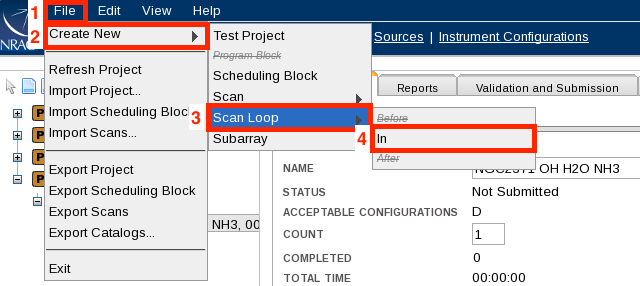 |
| Figure 39: Creating a loop. |
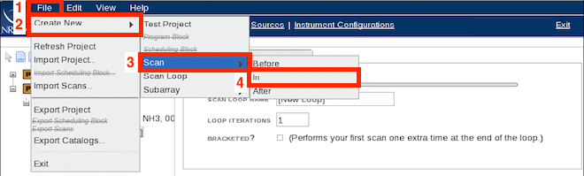 |
| Figure 40: Creating a scan within the loop. |
Within the [New Scan] entry fields, click the Import button in the Target Source field; this will bring up the VLA catalog by default. Select the calibrator you want to use for this tutorial, J0741+331. Rather than scrolling through the entire list of calibrators, you may select the RA position to narrow the search (in this case RA 07, see Figure 41A).
 |
| Figure 41A: Importing a calibrator source. |
With the OPT 1.31 release there is the ability within the scan to be able to filter the results. As seen in Figure 41A, you have to scroll a fair distance within the RA 07 sources to find J0741+3112. However, if you click on the option to Filter Sources, you are presented with the display as seen in Figure 41B. You click on import (1) as above, then click on Filter Sources. A new window appears that allows you to refine your search. You still need to enter a Source Catalog (2) and a Source Group (3 - if there is one). You can then enter a name of a source (4), or the RA and Dec of a known source, or do a radius search of n degrees based upon the RA and Dec positions. The filtered results are then displayed and you can select the source you want (5). Finally, click on Change (6) to import the selected source.
 |
| Figure 41B: Using the filter to import a calibrator source. |
To import the resource, click the Import button in the Hardware Setup field, select the project's resource catalog, and there you will see the L-band spectral setup you created (see Figure 42). Note that with the 1.31 release you have the option to also filter the Resources by observing band and/or sampler setup. This is useful if you have a large resource catalog to work through. For this example we only have two sources to choose from, so filtering the resource list makes no sense.
 |
| Figure 42: Importing a resource from project catalog. |
To finalize this calibration loop scan, select the "Calibrate Complex Gain (A and P)" intent, and uncheck the "Observe target" since this is a calibrator, and set the scan length to a reasonable LST duration (e.g., 1 minute).
The next scan, for the science target, can be created by clicking the Page-+ icon (the third icon at the top), which copies the scan into a new scan with the hardware setup and source from the previous scan. Change the source to the science target by selecting your source catalog in the dialog box and adjust the Scan Timing to 00:07:30 Duration (LST) (see Figure 43). Note the Observe Target intent is the default scan intent. If you make a mistake, a scan or an entire SB can be deleted or cut by selecting it and clicking on the Scissors icon (the fourth icon at the top).
 |
| Figure 43: A science target scan. |
To duplicate the science target scan, click on the Copy icon (the fifth icon at the top), and paste it with the Paste icon (sixth item at the top) to increase the duration of the science target to twice 7.5 minutes. Finally, select the calibrator scan and copy/paste it to the last scan in the loop, this time by selecting from the menu Edit → Copy STD: J0741+3312, then click the last scan and select from the menu Edit → Paste After STD: NGC2371 (see Figures 44 and 45).
 |
| Figure 44: Copy scan STD: J0741+3312. |
 |
| Figure 45: Paste After scan STD: NGC2371. |
Now we will create a similar loop in K-band, and place it so it is observed before the L-band scans.
Select the L-band loop (rename it to "L-band loop" or something descriptive) and select from the menu File → Create New → Scan Loop → Before, and give the new loop a name, e.g., K-band loop. Since we want the K-band loop to run 15 times, set the Loop Iterations to 15 (see Figure 46).
 |
| Figure 46: The K-band loop settings. |
In the K-band loop we want to create a science target scan of 7 minutes and a complex gain calibration scan of 1 minute, similar to the steps for the L-band loop, except using the K-band resource that was created for the Hardware Setup.
Since K-band observations require reference pointing calibrations, place another complex gain calibrator scan before the K-band loop (see Figure 47). Be sure to import the K-band setup for the Hardware Setup and use the "Calibrate Complex Gain (A and P)" scan intent for the complex gain calibrator scans.
|
|
| Figure 47: Filling the K-band loop. |

Because K-band is high frequency, we will be adding reference pointing scans (see below). We will select the Apply Last Reference Pointing setting for all K-band scans, except for the pointing scan itself. Note we can extend the complex gain calibrator scan before the loop and use it as a bandpass calibrator if we decide to do so. However, 3C48 is bright enough and does not differ much in flux density with this source in K-band, so we will use 3C48 for bandpass calibration and benefit from the known spectral slope of this standard flux calibrator in determining the bandpass.
Before the first calibrator outside the loop, we need to add a pointing scan (see Figure 48). And because we are switching from 8-bit to 3-bit after the pointing, another setup scan is required. We add two scans of the calibrator: the first scan should be a pointing scan with scan mode selected to be Interferometric Pointing and an initial duration of 3 minutes (may need to be increased later) using the X-band pointing resource from the NRAO defaults catalog and the pointing target (which fortunately again is J0741+3112). Furthermore, make sure there is no "Apply Last" selected in the reference pointing column.
 |
| Figure 48: The Reference pointing scan using the complex gain calibrator source with the adjusted time on source of 7 minutes. |
The second scan, which is another setup scan after the 8-bit resource pointing scan but before the 3-bit K-band gain calibration scan, should apply pointing and use the K-band resource with a setup intent for a duration of 30 seconds (see Figure 49).
 |
| Figure 49: The basic science scan sequence starting with the pointing scan and the requantizer setup scan before the gain calibration scan. |
Start-up Overhead
Figure 49 shows the science part of the observation. Now we should allow for the start-up overhead, flux density, and bandpass calibration. The flux/bandpass calibration is best placed at the start or at the end of the observation as it typically requires long slews away from the region of interest. Here we chose to do flux density calibration at the start of the observation using 3C48. Other examples are given in the extensive documentation throughout the OPT manual and the Guide to Observing with the VLA. The sequence to follow from the start of the observation to the first science scans is as follows:
| Default Resource Setup at the Start | Scan Time | Intents and Notes |
|---|---|---|
| L-band setup on first source (3C48) | 3 minutes | setup scan (set 8-bit attenuator levels) |
| K-band setup on first source (3C48) | 1 minute | setup scan (set 3-bit attenuator levels) |
| X-band pointing setup on first source (3C48) | 1 minute | setup scan (set 8-bit attenuator levels) |
| Flux and Bandpass Calibrator Scans | Scan Time | Intents and Notes |
|---|---|---|
| X-band reference pointing on 3C48 | 7 minutes | Interferometric Pointing scan mode; Start-up includes initial setup scans plus the first calibrator or reference pointing scan to allow 10-12 minutes in total duration. When starting with reference pointing, a 12 minute (minimum) start-up is the best approach. |
| K-band 3-bit setup on 3C48 | 30 seconds | setup scan (setting requantizer levels) when switching from 8-bit (X point) to 3-bit (K), apply last (reference pointing) |
| K-band bandpass and flux on 3C48 | a few (3) minutes | flux density scale, bandpass, complex gain, apply last (reference pointing) |
| L-band bandpass and flux on 3C48 | a few (3) minutes | flux density scale, bandpass, complex gain, apply last (reference pointing) |
| Science scans to follow | science target bracketed by the complex gain calibrator |
If the four flux density and bandpass scans are moved to the end of the observation, the resource setup at the start would be using the pointing source and an additional pointing scan on that source for 7 minutes. Examples can be found in the OPT Manual and the Guide to Observing with the VLA. The sequence in the table above is shown in Figure 50.
 |
| Figure 50: The resource setup and flux and bandpass scan overhead at the start of the observation, before the basic science scans. |
Now that the observing structure is in place, click on the SB name to enter the scheduling parameter within the Information tab. In the hypothetical proposal for this project, the LST range for this source to be above 25 degrees elevation was calculated to be between 02h16m and 18h51m. The earliest LST start time for this observation is 02h16m, but as this block is 2.5 hours long, the latest LST start time is 16h31m (which follows from the latest LST allowed, 18h51m, minus 2h30m for the length of the block). Enter this in the Information tab for the LST start range (02:15 and 16:30). Finally, select the weather conditions for the highest frequency band used in the SB (K-band), i.e., 7 m/s for wind and 10.0 degrees for the API upper limits to start this SB (see Figure 51).
 |
| Figure 51: The dynamic scheduling starting conditions for this SB for LST start range and weather for the highest frequency band in the SB. The set up scans for slew to area of sky and attenuation set up are the scans in the red block; reference pointing scans and flux density / bandpass calibration scans are in the blue block; complex gain calibration and science target scans are in the green block. (Click to enlarge) |
Fine Tuning
Click on the Reports tab to see how this SB would perform for the average start time (12:52:30, or any other time selected within the assumed LST start range on the Reports tab). The window at the bottom will show an error and the scan listing (third table down the main window) will show many red rows (see Figure 52).
 |
| Figure 52: The scan rows in red indicates an error condition with the scan (source elevation below the horizon). |
For the first scan, and the setup scans to follow, this is normal and nothing to worry about; but it should be clear that for the assumed starting time of 12:52 LST that 3C48 has already set below the horizon. The Guide to Observing with the VLA shows that 3C48 is only up until about 08:33 LST for the minimum elevation limit (10 degrees), and will be below the anticipated 25 degrees elevation limit after about 07h LST. Return to the Information tab and use 06:40 as the latest LST start (to account for the first 20 minutes of time spent on 3C48), and go back to the Reports tab. Another error appears, this time on the pointing scan which requires 2:30 minutes on source after any necessary slewing. We allocated a duration of 3 minutes, but more than 30 seconds is spent on slewing from 3C48 to the first source (see the red scan row in Figure 53).
 |
| Figure 53: The reference pointing scan on J0741+3312 is too short to perform the antenna pointing. |
In this particular case the software chooses the shortest way, clockwise (CW), to go from Az 280° (where 3C48 is at the LST start time) to the rising gain calibrator at Az 440°. The antenna array should be directed counter-clockwise (CCW) to make this slew happen from Az 280° CCW to Az 80°(=440°). To achieve this, select CCW wrap for the relevant (8th) scan (see Figure 54) on the gain calibrator and add about 5 minutes to the total time to allow for a 200° slew at 40° a minute (the Azimuth slew rate of the telescopes). These errors are now gone in the Reports tab, and ample time is left for the pointing scan.
 |
| Figure 54: Selecting the wrap for a scan. |
Try other LST start times in the start range, watch for errors on particular scans, and fix them if they appear. Make sure to stay within the allocated time (2h30m) and modify the schedule, if necessary, to achieve this criteria. In this case the total time is 2:45 so 15 minutes must be cut, for example, by taking 40 seconds off the K-band target scan and 20 seconds off the K-band calibration scan (one minute per loop, 15 loops). Other choices are also possible as long as you can still detect your calibrator and perform other calibration scans. Go back to the Reports tab and play around with LST start times and look for errors, e.g., short on source times (less than 20 to 40 seconds). Finally, go to the Validation tab, validate and submit (Figure 55).
Note that with the release 1.31 there is an option for you to opt out of COSMIC-SETI (information on COSMIC-SETI). By default this box is always checked, meaning that COSMIC-SETI will get the raw data plus the metadata (source name, position, observing frequency, etc.) from your observing. Opting out means that while COSMIC-SETI will still get the raw data, none of the metadata are provided, which renders the raw data useless.
 |
| Figure 55: The Validation tab. (Click to enlarge.) |
If you have problems that you cannot fix yourself or with help of a colleague, please feel free to ask the NRAO Hepdesk.
Single-band Continuum and Polarization Tutorial
In this Observation Preparation Tool (OPT) tutorial, we will create an S-band continuum polarization scheduling block (SB) to be observed in D-configuration. There are many guidelines to consider when setting up an observation.
RCT User Interface Update
The Resource Catalog Tool (RCT) had a recent UI update. This tutorial follows the steps for setting up resources using the Manual mode (aka the old RCT UI). We now have four distinct options in the RCT: Spectral Line, Frequency Sweep, Continuum, and Manual. The OPT manual has been updated to reflect the new RCT, sections of which can be found in the Resource Catalog Tool section in the OPT manual.
Guidelines for Observing S-band Continuum Polarization in D-configuration:
(For more details on the following topics, refer to the Guide to Observing with the VLA.)
- S-band Instrument Configuration: Select an NRAO default resource or create your own resource.
- Calibrators:
- complex gain (amplitude and phase)
- flux density scale
- bandpass and delay
- polarization leakage (D-term)
- polarization angle
- Calibration Strategy:
- Cycle time for appropriate phase calibration for low frequency observing in D-configuration.
- Placement of the polarization calibrators within the SB.
- LST Start Range:
- Within the SB, setup the S-band resource in one of the satellite-free zones. (Recommended, but not required.)
- Avoid elevations greater than 85°.
- Avoid elevations less than 40° (if possible) to avoid antenna shadowing. (Recommended, but not required.)
- Check to see if an antenna wrap is required.
All questions regarding this tutorial or observation setup in general, should be submitted to the NRAO Science Helpdesk under the VLA Observing department.
Accessing the OPT
To access the OPT and its suite of tools, login to the my.nrao.edu portal, or register if you have not already done so. Once you have logged in, click on the Obs Prep tab near the top and then click on the text Login to the Observation Preparation Tool (OPT) (see Figure 1).
|
|
|---|
| Figure 1: Accessing the OPT and its suite of tools. |

Instrument Configurations
Once you have logged into the OPT, click on Instrument Configurations at the top to access the Resource Catalog Tool (RCT) (see Figure 2).
|
|
|---|
| Figure 2: Accessing the Resource Catalog Tool. |

On the left-hand side within the RCT, you will see a tree titled NRAO Defaults. Open this tree by clicking on the + symbol, then select the group of defaults titled up to 2x1GHz (8bit). Figure 3 shows the first page of all NRAO Default resources where you can find your S-band resource to use (S16f5DC). By selecting the listed groups [Pointing setups, up to 4x2GHz(3bit), up to 2x1GHz(8bit)] you can narrow down the list of available default resources based upon their properties of pointing, 3-bit, or 8-bit resources.
|
|
|---|
| Figure 3: NRAO Default resources. (Click to enlarge) |

Please note that from previous NRAO Default resources there have been some changes. The first is in the description there is the "doNotChange". Default NRAO resources should not be changed by the user; if the NRAO Default does not meet your science requirements, you should create your own custom Continuum science resource, the instructions for which can be found in our documentation on Custom Type Continuum Setup.
Second, there is at the end of the resource description "dflt RFI blank". NRAO has incorporated RFI blanking to help minimize RFI. With a custom resource you can turn RFI blanking on or off. Please read our documentation on RFI blanking to learn more about this option.
For low frequency observing in D-configuration, we generally recommend a 5 second correlator integration time. The S-band resource S16f5DC (decoded in Table 1 below and seen above in Figure 3) is an appropriate choice for the observation we will be creating. Once we begin building the SB within the OPT, we will import the S16f5DC resource into the scans. Note that to see more details of the resource, you may click on the icon which looks like a blue square with a yellow bar/pencil. If needed, more information can be found in the RCT section of the OPT manual.
| S-band default resource S16f5DC | |
|---|---|
| S | frequency band |
| 16 | number of subbands (8 subbands per baseband) |
| f | full polarization (RR, LL, RL, LR) |
| 5 | correlator integration time in seconds |
| DC | suitable array configurations |
Table 1: The S-band default resource decoded.
Sources
If you have a successful proposal, about a month before the start of the proposed array configuration, your project will be imported into the OPT by NRAO staff. During this import process, a catalog of the proposed and accepted sources will be imported into the Source Catalog Tool (SCT). If you are working through this tutorial before your approved project has been made available within the OPT, this tutorial will show you how to create your own source catalog; more detail about the SCT can be found in the OPT manual.
To access the SCT, click on Sources at the top of the screen, as shown in Figure 4.
|
|
|---|
| Figure 4: Accessing the Source Catalog Tool (SCT). |
Create a New Source Catalog
To create a new source catalog, select File → Create New → Catalog (see Figure 5) then name the catalog. (Note that you may share the source catalog with others by adding them as co-I's using the Properties tab; co-I's must have a my.nrao.edu account.)
|
|
|---|
| Figure 5: Creating a new source catalog. |

Create a New Source
Once you have created the source catalog, you may add or create new sources in it. To create a new source within the catalog, select File → Create New → Source (see Figure 6).
 |
|---|
| Figure 6: Creating a new source within the catalog. |
Now you name the source and enter in the RA and Dec of the science target coordinates. For this tutorial we will be observing 3C75, a binary black hole system.
- RA: 2h 57m 42.63s
- Dec: 6d 1' 4.8"
You may copy/paste the above coordinates into the RA and Dec fields under Source Positions (see Figure 7). Be sure to hit tab or click outside of the field to allow the SCT to take the entry. Note that the SCT, RCT, and OPT do not have a save button; any changes that are made are automatically saved. Please note that if you make changes to a source position or an instrument configuration after it has been imported into a scan within the OPT, those changes will not automatically propagate throughout the scans. Instead, the resources must be re-imported into the OPT.
 |
|---|
| Figure 7: Enter source name and coordinates. |
Select the Images tab (see Figure 8) to help you determine an initial LST range of the SB. 3C75 is visible at the VLA from about 21:30-08:30 LST. This source time range is different from what we define as the LST start range of an SB. We will adjust the LST start range once we have created the SB. Note the LST start range will be restricted by other sources, i.e., the flux density calibrator.
|
|
|---|
| Figure 8: Images tab of 3C75 showing the elevation curve. |

Selecting Calibrators
Complex Gain Calibrator (Amplitude and Phase)
To search for an appropriate complex gain calibrator within the VLA calibrator database, we will use the Advanced Search feature located on the left-hand side. Select VLA from the Source Search, this enables searching the VLA calibrator database. Next, select the Cone Search parameter; enter in the RA and Dec of 3C75 (2h 57m 42.63s and 6d 1' 4.8") or select the source from the catalog you created, then widen the search radius to 15.0d (suggested maximum angle for gain calibration at low frequency), and click on the Search button. See Figure 9 for a visual guide.
With the update to 1.31 a Sky Map option has been included for the Cone Search parameters box. After entering the RA and Dec and clicking the Search button, when you click on the Sky Map icon a Sky Map will be displayed with the RA and Dec of the source in the center; this makes it easier to visualize the position of the calibrators in the sky relative to the target.
 |
|---|
| Figure 9: Advanced Search in the SCT. |
The results of the search are shown below in Figure 10. If you hover your mouse over the word Details within the SCT table, you will see the fluxes and structure codes for the known bands in the corresponding array configurations. The first calibrator in the list is not sufficient since it does not have information for the low frequencies (only Q-band). The second calibrator in the list, J0259+0747, has information for L- and C-band. Since S-band is in between these two frequency ranges, J0259+0747 can be considered and will be used in this tutorial as a complex gain calibrator. Instructions on how to choose the best complex gain calibrator can be found in the Low Frequency Strategy guide. For this particular tutorial, it is reasonable to choose J0259+0747 since it can also be used as a polarization leakage calibrator (a polarized D-term calibrator). More details regarding polarization leakage calibration will be explained later.
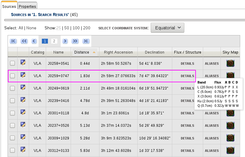 |
|---|
| Figure 10: Selecting the complex gain (amplitude and phase) and polarization leakage calibrator. |
Flux Density Scale Calibrator
When selecting a flux density scale calibrator, you must choose from one of the standard 3C calibrators: 3C48, 3C286, 3C138, 3C147, and 3C295. The SCT contains a list of these 3C calibrators. Each of these 3C calibrators, except for 3C295, have models in CASA and AIPS. You can see the list by opening the tree labeled VLA (located on the left-hand side) and then select VLA Flux Cal (see Figure 11).
 |
|---|
| Figure 11: The standard VLA flux density scale calibrators, |
The structure code and the proximity of the flux density scale calibrator to the science target is not as important as when choosing the complex gain calibrator. The flux density scale calibrator should be up, have a similar LST range as the science target, and relatively close to minimize the overhead of slewing. If we do another Advanced Search centered on the science target (as explained in Figure 9 above), with a wider cone radius of 40.0d, we will find 3C48 as the closest option (32.9° from the science target). Click on the icon (blue square with a yellow bar/pencil) to the left of the source name to access the Images tab. There you will see the LST range is about 19:00-08:20, similar to 3C75 (21:30-08:30 LST).
Bandpass & Delay Calibrator
In most cases, the standard flux density scale calibrators can double as the bandpass and delay calibrator. We generally recommend using a very bright calibrator for the bandpass calibration. For this observation, we will use 3C48 as the bandpass and delay calibrator since it is very bright in the lower frequencies.
For more details regarding the complex gain, flux density scale, bandpass, and delay calibrators, refer to the Calibration section of the VLA observing guide.
Polarimetry
Since we want to image in Stokes Q and U, the instrumental polarization can be determined through observations of a bright calibrator source spread over a range in parallactic angle (> 60°). In order to determine the leakage term (i.e., the polarization impurity between the R and L polarizations, also known as the "D-term") and calibrate the absolute polarization angle, we must choose the appropriate polarization calibrators.
Polarization Leakage Calibrators
To help determine the instrumental polarization and/or to check if the instrumental polarization was properly calibrated or removed during post processing, we will use an unpolarized D-term calibrator, J2355+4950 and a polarized D-term calibrator, J0259+0747. The source J2355+4950 was chosen from Table 7.2.3 in the Polarimetry section within the VLA observing guide. We will give this source the calibrate complex gain (amplitude and phase) scan intent to ensure that, if the VLA pipeline is used to calibrate the data, its observation will be self-calibrated and can be used as an instrumental polarization calibrator if further processing is needed.
As discussed in the section above regarding the selection of the complex gain calibrator, we determined J0259+0747 is appropriate as a polarized D-term (polarization leakage calibrator) since it is known, from a recent calibrator survey for the VLA Sky Survey that included polarization information, to be 5% polarized.
For this observation, we will observe J0259+0747 for determining the instrumental polarization. An unpolarized D-term calibrator is needed only if the parallactic angle coverage is less than the recommended 60°, i.e., for short duration SBs. In this case we use the unpolarized calibrator J2355+4950 to verify the polarization leakage was correctly removed after calibration.
Polarization Angle Calibrator
3C48 will be used as the polarization angle calibrator since it has a well known polarization angle at low frequencies (S & C-band). Note its polarization fraction is only high enough to be a reliable polarization angle calibrator above 2.5 GHz.
For more details regarding the polarization calibrators, refer to the Polarimetry section of the VLA observing guide.
Observation Preparation
Now that we have chosen one of the NRAO Default S-band resources, and determined the calibrators, we can create the SB.
To access the OPT, select Observation Preparation located near the top of the screen (see Figure 12).
 |
|---|
| Figure 12: Accessing Observation Preparation. |
Create a Test Project
In order to create the SB, we will need to create a New Test Project.
Select File → Create New → Project In the pop-up box click on "TEST PROJECT" then the Add button (see Figures 13A & 13b).
if you have an accepted proposal, but it is not yet available within the OPT, you may create a Test Project to begin working on the SB(s). After the project has been made available within the OPT, you may then copy/paste the SB you've been working on into the project under the corresponding Program Block (PB).
| Figure 13A: Creating a new Project. | Figure 13B: Making a new Test Project. |
The project tree is made up of three levels:
- P: Project level contains the project code, PI, co-I's, and total allocated time.
- PB: Program Block level contains the allocated time per PB, scheduling priority, Acceptable Configurations, Linked Scheduling Blocks, list of Scheduling Blocks (SBs), and a list of Execution Blocks (once an SB has been observed).
- SB: Scheduling Block(s) contain scans with assigned sources, resources, duration (in LST), and scan intents (i.e., Setup, Observe Target, Flux Density, etc.).
Now that the Test Project has been created, you may give it a name and/or share with other co-I's, if you wish.
Edit the PB
Next we will assign the PB an array configuration; this option is only available for test projects. Under the PB level of the Project, select the D under Available Configurations and drag it to the left under the Acceptable Configurations (see Figure 14). At this point you can also name the PB.
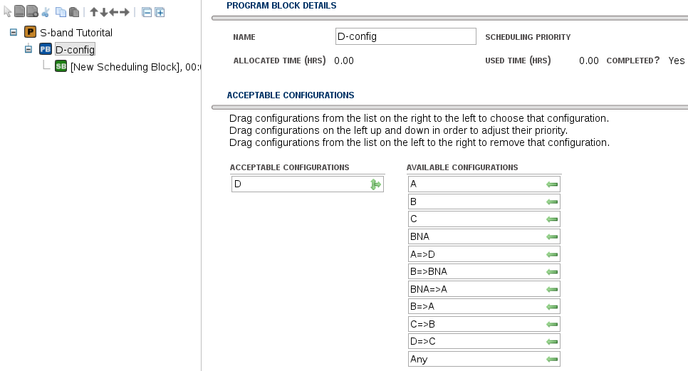 |
|---|
| Figure 14: Assigning D to acceptable configurations and naming the PB |
Create a New SB
When creating a Project, an empty SB is automatically generated. You may use this SB or create a new SB.
To create a new SB, select File → Create New → Scheduling Block (see Figure 15).
| Figure 15: Creating a new scheduling block (SB). |
SB Information Tab
In the Information tab of the SB we can name the SB, set a preliminary LST start range of 21:30-08:30 (from the science target source, 3C75), and select the default S-band wind and Atmospheric Phase Limit (APL) constraints (see Figure 16). Recall that we will adjust the LST start range once we have finished creating the scans within the SB as, at a minimum, we would have to shorten the end time with the length of the SB.
With the update to 1.31 the Weather Constraints table has been changed to allow for alternate atmospheric phase limit values if you are planning to self-calibrate.
 |
|---|
| Figure 16: Information tab of the SB. (Click to enlarge) |
SB Setup Overview
Next we will create the scans within the SB. We should first discuss, however, the order of the scans to be created, their sources, and corresponding scan intents.
All SBs must start with at least a 1 min setup scan for all resources to be used in the observation; this will set the attenuator levels in the correlator. These levels will be set and remembered for the entire duration of the observation. Following the 1 min setup scan there should be at least a 9 min calibrator scan. This is to allow for the minimum recommended start-up for low frequency observing to be a total duration of 10 min. This start-up is to ensure plenty of slew and on source time for the first calibrator scan.
For this S-band observation, we will start with a dummy slew scan of 9 min using a different resource (e.g., C-band), followed by the 1 min setup scan for the S-band resource and then a 5 min scan on the first calibrator (in this case the flux density scale calibrator). The extra dummy slew scan is to allow the antennas to slew to one of the satellite-free zones (see Table 2) and then set the attenuator levels for the S-band resource. This 9 min duration assumes a worse-case-scenario in that the starting position for the antennas could be at its furthest from where they need to be. If this is the case, it can take up to 9 min for the antennas to slew to their destination. The AZ and EL slew rates of the antennas are 40°/min and 20°/min, respectively. Later in this tutorial we will work on adjusting the LST start range to accommodate this special start-up sequence.
| Satellite-free Zones |
|---|
| 250° < AZ < 330° and EL > 30° |
| 45° < AZ < 90° and EL < 60° |
Table 2
For more details regarding the setup scans and setting up in the satellite-free zones, refer to the 8/3-Bit Attenuator and Requantizer Gain Setup Scans in the VLA observing guide.
Table 3 below provides a basic outline of the scan duration, sources, resources, and scan intents to be used in the SB.
| Scan Duration | Source | Resource | Scan Intent(s) |
|---|---|---|---|
| 9 min | 3C48 | C-point | Setup Intent; slew to satellite-free zone |
| 1 min | 3C48 | S16f5DC | Setup Intent; set up attenuation in satellite-free zone |
| 5 min | 3C48 | S16f5DC | Calibrate Flux Density, Calibrate Bandpass, Calibrate Delay, Calibrate Polarization Angle |
| 4 min 30 sec | J2355+4950 | S16f5DC | Calibrate Complex Gain (amplitude and phase) |
| 6 min | J0259+0747 | S16f5DC | Calibrate Complex Gain (amplitude and phase), Calibrate Polarization Leakage |
| Loop x7 | |||
| 15 min | 3C75 | S16f5DC | Observe Target |
| 1 min 15 sec | J0259+0747 | S16f5DC | Calibrate Complex Gain (amplitude and phase), Calibrate Polarization Leakage |
Table 3: Basic outline of the SB.
Note that while the order of the scans is important, the order in which the scans are created is up to the observer. For example, some may prefer to create the science target scan(s) and the calibrators scans first, then create the setup scans. The OPT allows scans to be moved after creation.
Create Scans
To create a new scan, select File → Create New → Scan → In (see Figure 17).
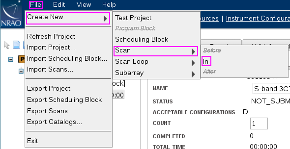 |
|---|
| Figure 17: Creating a new scan within the SB. |
Once the scan has been created, we will change the name of the scan, import the source and resource, adjust the duration of the scan, and select the appropriate scan intents.
Source Import
To import the source, select Import (under Target Source), select VLA under Source Catalog, and you may narrow the options by selecting VLA Flux Cal under Source Group, then select either 3C48 or 0137+331=3C48, then select Change (see Figure 18).
New with 1.31 is the ability to filter your search. This is particularly handy if you are searching in the VLA catalog a source group with sources based on either RA or Dec positions. As there are many sources in the group, filtering the search by RA or Dec value can save time. In this example the VLA Flux Cal group is being accessed, which has few sources, so filtering this group isn't necessary.
 |
|---|
| Figure 18: Importing a source from the VLA calibrator catalog. |
Resource Import
To import the resource, under Hardware Setup select Import ; the default NRAO resources have been configured into four groups: All, 2x1GHz (8-bit), 4x2GH(3-bit), and Pointing setups. Since this is the dummy slew scan we will use the NRAO Default "C-point" resource. In the drop-down box for the Resource Group select Pointing setups, pick the reference pointing resource - here C-point - then select Change (see Figures 19A & 19B). Note there is nothing inherently special about choosing the C-band pointing default resource, other than it is not S-band and its default correlator integration time is 1 sec. We also could have chosen either "X-point" (both pointing resources have a 1 sec correlator integration time) or "L16f5DC" (the 5 in the name indicating a 5 sec correlator integration time).
With 1.31 you also have the ability to filter your resource by name, and/or observing band, and/or sampler. If you select a resource that does not have a sampler, e.g., L-band 3-bit, no resource will be returned. Also note that you can select multiple observing bands and samplers, e.g., C-band and X-band 3-bit and 8-bit, and a list of the resources will be returned that match these parameters. In this SB, you are selecting one of the two NRAO default reference pointing scans, of which there are only two resources, so it isn't necessary to filter the results.
 |
||
| Figure 19a: Importing a pointing resource from the NRAO Defaults. (Click to enlarge) |
Figure 19b: Selecting a pointing resource from the NRAO Defaults. |
If you haven't done so already, change the name of the scan to something that indicates what it is. This is not required, but can be helpful. The Scan Timing should be changed to 9 min to allow for plenty of slew time into one of the satellite-free zones, and change the Intents to use Setup Intent and uncheck the Observe Target intent (see Figure 20). Note that the Observe Target intent should only be used for the science target scans. An Observe Target intent selected for a setup scan or a calibrator scan will cause problems with the VLA calibration pipeline.
 |
|---|
| Figure 20: Dummy slew scan parameters. |
Copy/Paste Scans
To create all subsequent scans, we can copy/paste a scan by selecting Edit → Copy STD: <scan name> and then select Edit → Paste → Paste After STD: <scan name> (see Figures 21 and 22).
| space | ||
|---|---|---|
| Figure 21: Copy selected scan. | Figure 22: Paste after selected scan. |
S-band Setup Scan
We now make changes to this new scan for the S-band setup scan. Edit the scan Name, change the Scan Timing to 1 min (the minimum time required for setting the attenuator levels in the correlator), and import the S16f5DC resource under the Hardware Setup (see Figure 23). Notice the selected Resource Group under the NRAO Defaults is "up to 2x1GHz(8-bit)" in Figure 23. This will narrow the search for the S-band resource we decided to use earlier in this tutorial.
 |
|---|
| Figure 23: S-band setup scan. |
Calibrator Scans
Flux Density Scale, Bandpass, Delay, and Polarization Angle
Next we will copy/paste the S-band setup scan to create the first calibrator scan. Follow the same steps as seen in Figures 21 and 22 above, then change the scan Name, the Scan Timing to 5 min, and edit the scan Intents by selecting calibrate flux density scale, calibrate bandpass, then click on More >>> to select calibrate delay and calibrate polarization angle. Remember to uncheck setup intent (see Figure 24).
| Figure 24: Flux density scale, bandpass, delay, and polarization angle calibrator scan. |
Complex Gain (amplitude and phase) and Polarization Leakage
Following 3C48 will be a rather long duration scan of the secondary complex gain calibrator J2355+4950. The long duration on this calibrator scan is to ensure plenty of slew and on source time since this source is many degrees away from 3C48. The on-source time is determined by the need to obtain sufficient signal-to-noise per channel to solve for instrumental polarization. Copy/paste the flux calibrator scan, edit the scan Name, update the Target Source by importing J2355+4950, adjust the Scan Timing to 4.5 min, and select "Calibrate Complex Gain (A and P)". Remember to uncheck the other calibrator intents that were included from the copy/paste.
Next we will add another rather long scan (6 min) for the primary complex gain calibrator to ensure plenty of slew and on source time. Then we create the loop containing a science target scan and another primary complex gain calibrator scan.
Creating a Loop
To create a loop proceeding the primary complex gain calibrator, select File → Create New → Scan Loop → After (see Figure 25), then you may either copy/paste a scan or create a new scan within the loop. To copy/paste a scan into the loop, select the scan you wish to copy (use the primary complex gain calibrator), then select the loop you wish to paste the scan into, and select Edit → Paste → Paste Into Scan Name (see Figure 26). Do this last step twice so we have two scans inside the loop: one for the science target scan and one for the primary complex gain calibrator scan.
 |
space |  |
|---|---|---|
| Figure 25: Create a loop following the primary complex gain calibrator. | Figure 26: Paste the scan into the loop. |
Next we will edit the first of the two scans inside the loop to be the science target source 3C75. We can now import the source from the source catalog (see Figure 27) we made earlier in this tutorial. Then we will adjust the scan timing to 15 min, change the scan name, select Observe Target, and uncheck the calibrator intents.
 |
|---|
| Figure 27: Import science target source, 3C75. |
Next select the primary complex gain calibrator scan within the loop to adjust the scan timing to 1 min 15 sec.
Since we want the loop to be repeated 7 times, select the loop and edit the Loop Iterations field to 7. You may edit the name of the loop if you wish. Since the loop starts with the science target scan, do not select the option within the loop to bracket; if the loop were to start with the complex gain calibrator scan, then it would be appropriate to select the bracket option.
The basic layout of the SB is now complete.
LST Start Range
The next step is to adjust the LST start range to avoid the elevation limits, setup the S-band resource in one of the satellite-free zones, and avoid antenna shadowing (if possible).
To help determine an appropriate LST start range we will need to access the Reports tab of the SB. Click on the SB name and then select Reports near the top of the page (below the dark blue header). The Reports page shows the Instrument Configuration Summary, Time On Source Summary, and the Schedule Summary. We will adjust the assumed LST start to the earliest of the LST start range for 3C75 of 21:30 (click Update or hit return/enter on your keyboard) (see Figure 28). You may have noticed that, after clicking Update on the Reports page, the total duration of the SB updated (seen in the left-hand side next to the SB name). If you make a change to the length of a scan, you will need to click Update on the Reports page to force the OPT to recalculate the length of the SB.
 |
|---|
| Figure 28: Adjust the assumed LST start time on the Reports page. |
Finding the right LST start range is an iterative process by stepping through the LST start range in 5-30 min increments and then checking the Schedule Summary (bottom table on the Reports tab) to see how AZ and EL change, how slew time changes between sources/scans, and how on source time for each scan changes. We recommend at least 20 sec on source for science target and complex gain calibrator scans, and at least 40 sec on source for flux density scale, bandpass, and delay calibrator scans. Of course, more time on source may be required depending on the flux of the source and the signal to noise required for the science. When setting up your own observations, we recommend using the Exposure Calculator Tool (ECT) to help determine the appropriate time on source. This tutorial should not be used to help you determine the required time on source for your science.
Recall earlier in this tutorial the difference between the source LST range and the LST start range of an SB. If we set the assumed LST start to 08:30, you will see under the Schedule Summary table that all sources are below the VLA's horizon and the hard elevation limit of 8°. This illustrates the difference between what is meant by source LST range and LST start range.
If we set the assumed LST start to 06:00 and check the Schedule Summary, we see that all scans have an elevation greater than the recommended absolute lower elevation limit of 10°. Going through the iterative process of changing the assumed LST start and checking the Schedule Summary table, we will eventually determine the following:
- 21:30-00:55 LST is ok, however it does not setup the S-band resource within one of the satellite-free zones for the entire LST start range.
- 01:00-02:00 LST exceeds the upper elevation limit of 85°.
- 02:05-04:15 LST is the optimal start range. The S-band resource is setup in one of the satellite-free zones for the entire start range, upper and lower elevation limits are avoided, antenna shadowing is avoided, and all scans have the appropriate amount of time on source. With this LST start range, a clockwise (CW) wrap should be requested on the start-up scans (all setup scans plus the first calibrator scan).
Appendix
The SB in this tutorial was modeled after a real observation taken in D-configuration on 2018 Oct 04 UT. The data set can be downloaded from the NRAO Archive by typing in TDRW0001 into the Project (Proposal) Code field and then select TDRW0001.sb35624494.eb35628826.58395.23719237269 for download as either an SDM or an MS. The differences for the observed SB are as follows:
- Additional dummy slew scan at the start of the SB.
- A 30 sec requantizer gain setup scan for the S-band resource following the 1 min attenuator setup scan. The additional 30 sec requantizer setup scan is optional for 8-bit low frequency observations. For more details, refer to the 8/3-Bit Attenuator and Requantizer Gain Setup Scans within the VLA observing guide.
- A few extra and slightly longer scans on the primary complex gain calibrator in between two loops of the science target and the primary complex gain calibrator, causing the SB to be longer in total duration.
- LST start range used was 23:00-00:30 with a CCW antenna wrap request on the 3C48 scans. This was selected since it was in a low observing pressure range at the time of the observation. (A daily pressure histogram is posted on the Schedsoc Home Page.)
- S-band instrument configuration was modified to utilize one baseband to provide a decrease in the data rate, allowing for a smaller data set to be used for the VLA Data Reduction Workshop.
These subtle differences do not change the overall science goal of the observation, but is an example of the flexibility of setting up a low frequency observation for the VLA.
You may download and then import the xml file, S-band_tutorial.xml, into the OPT.


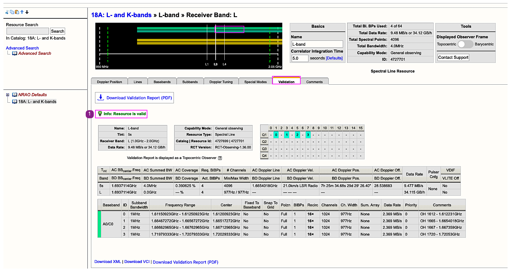
Connect with NRAO